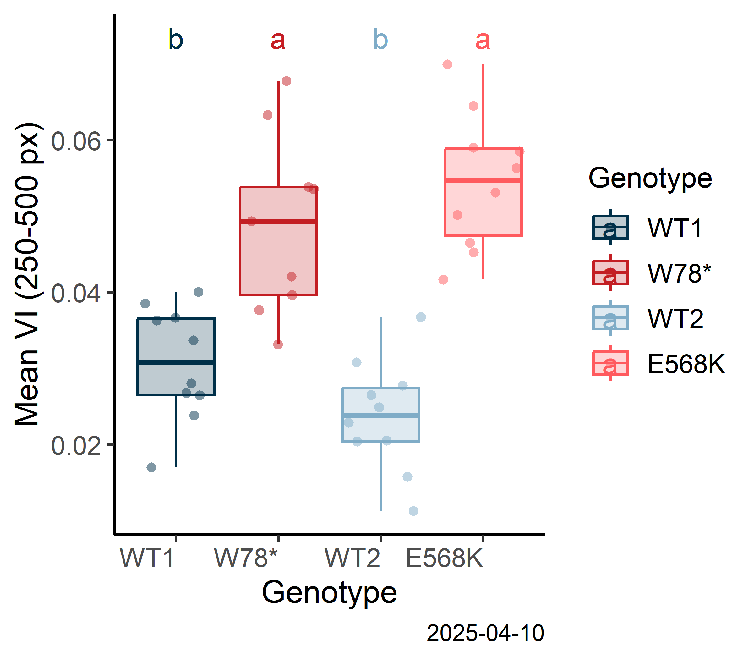
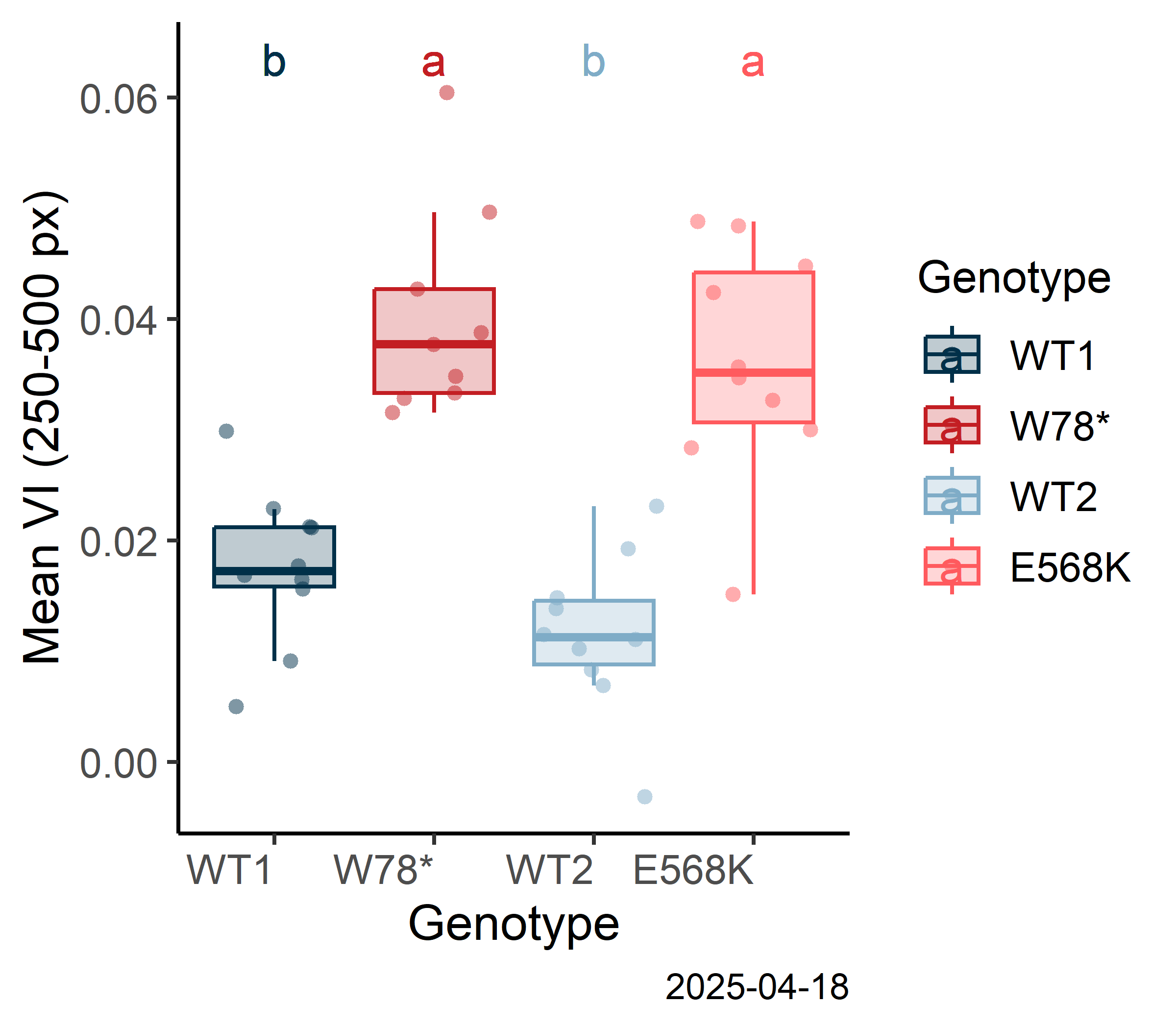

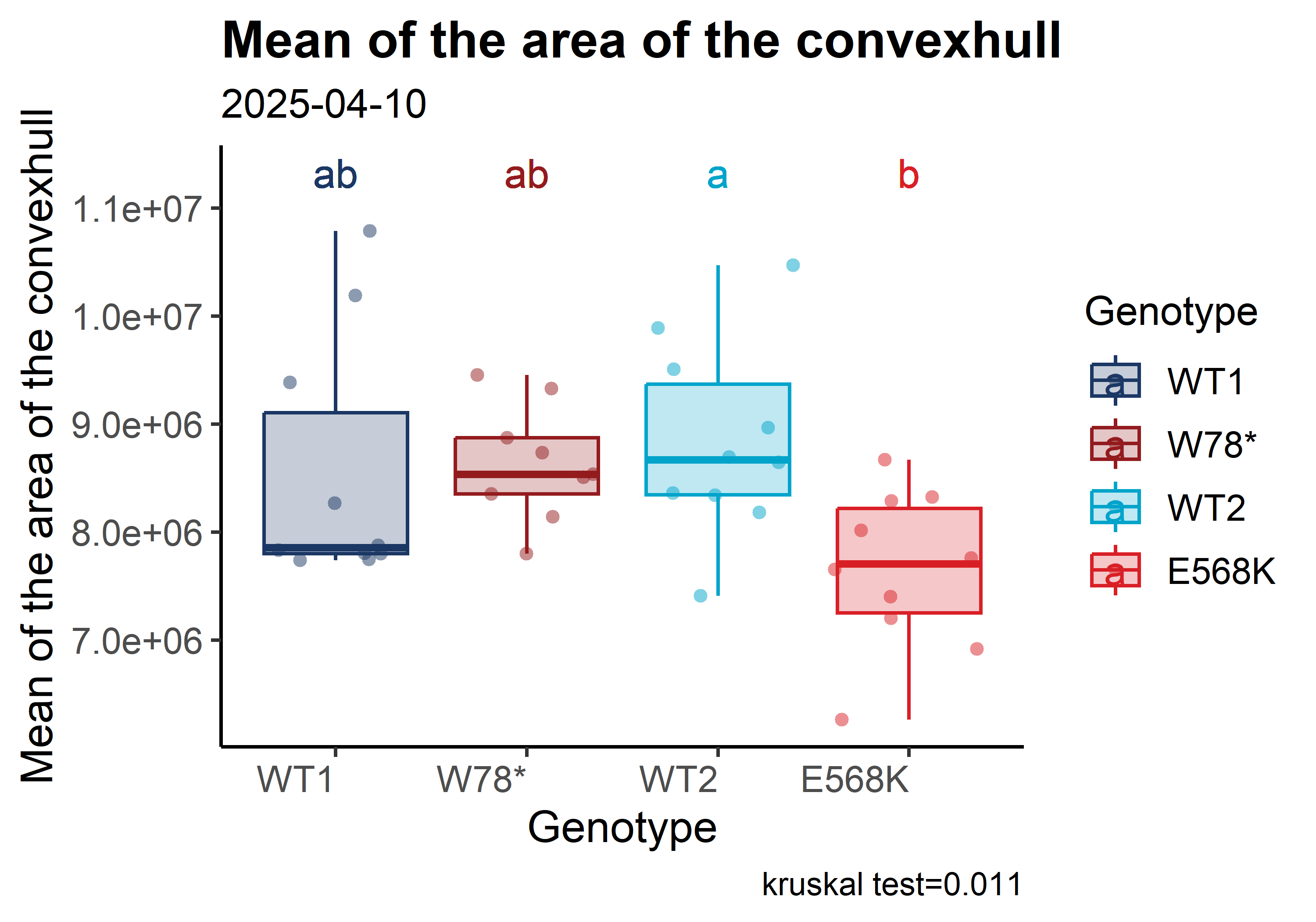
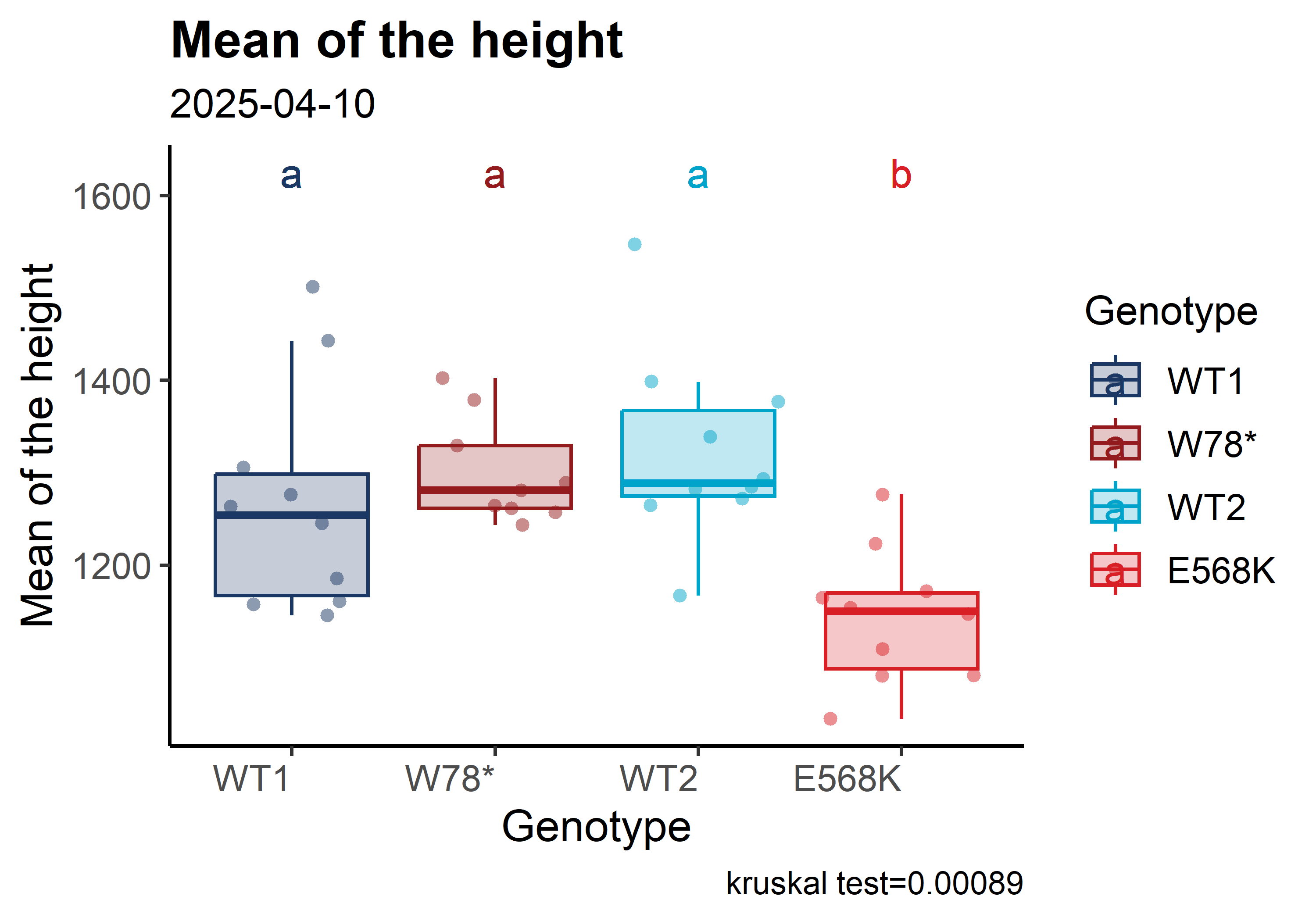
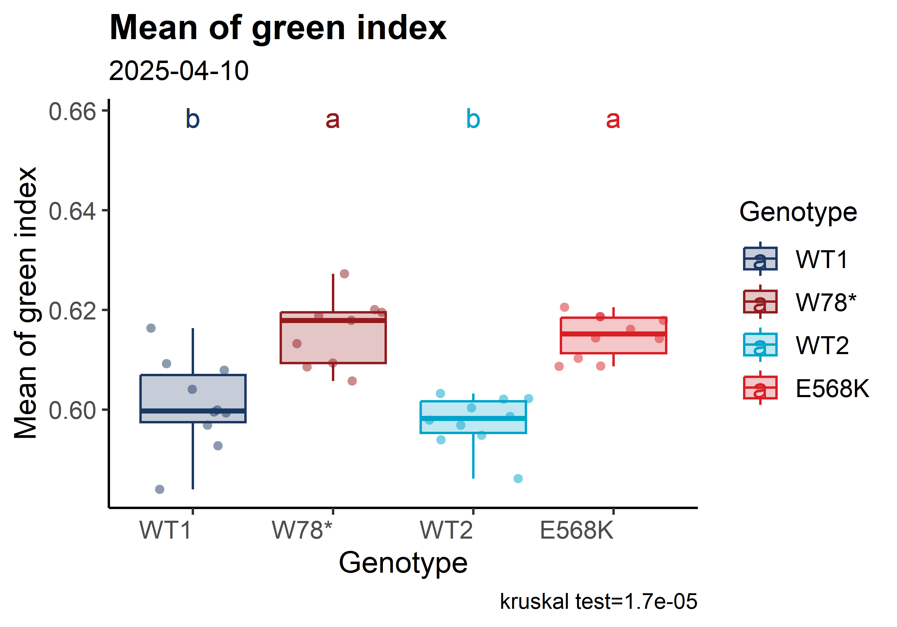
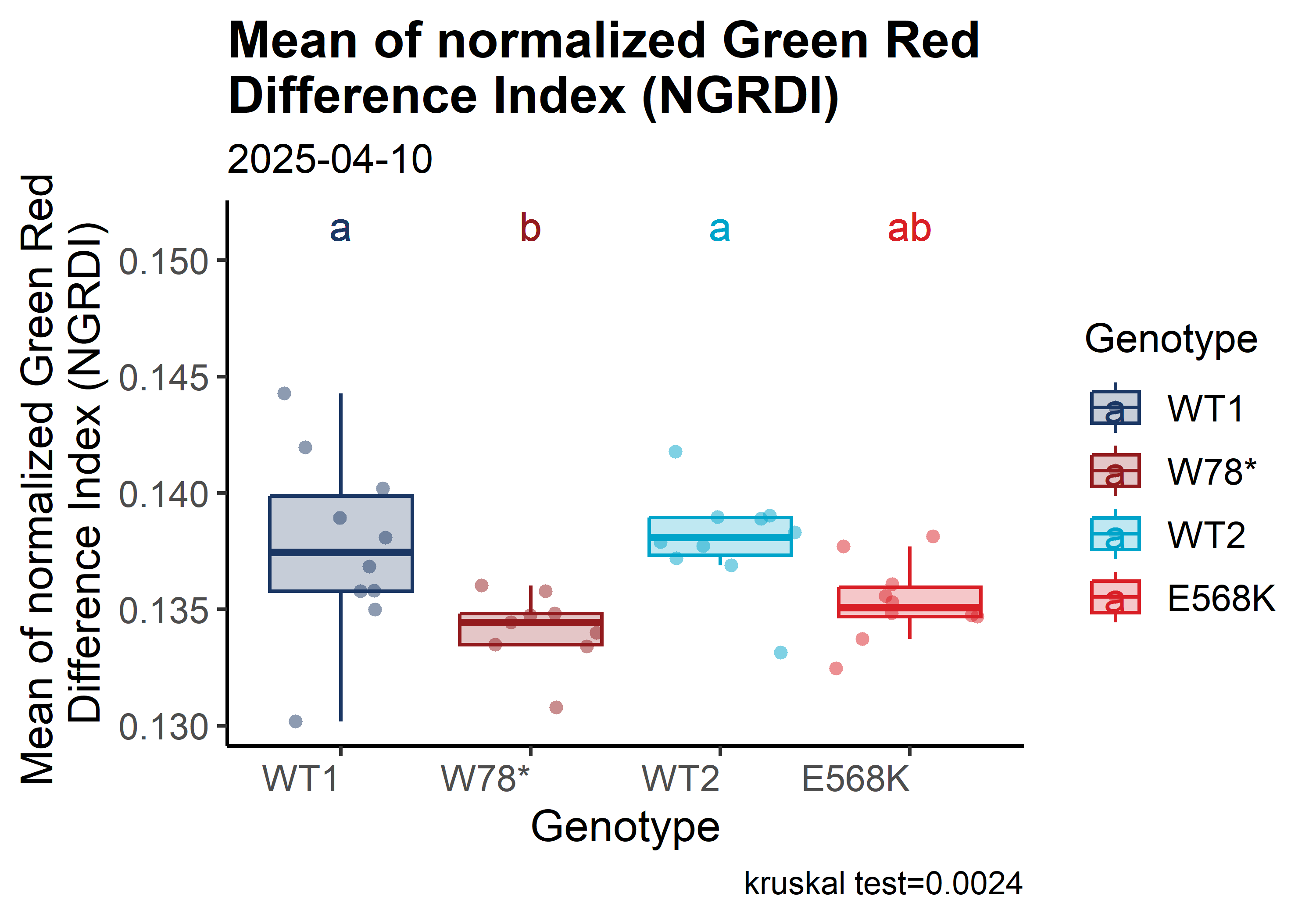
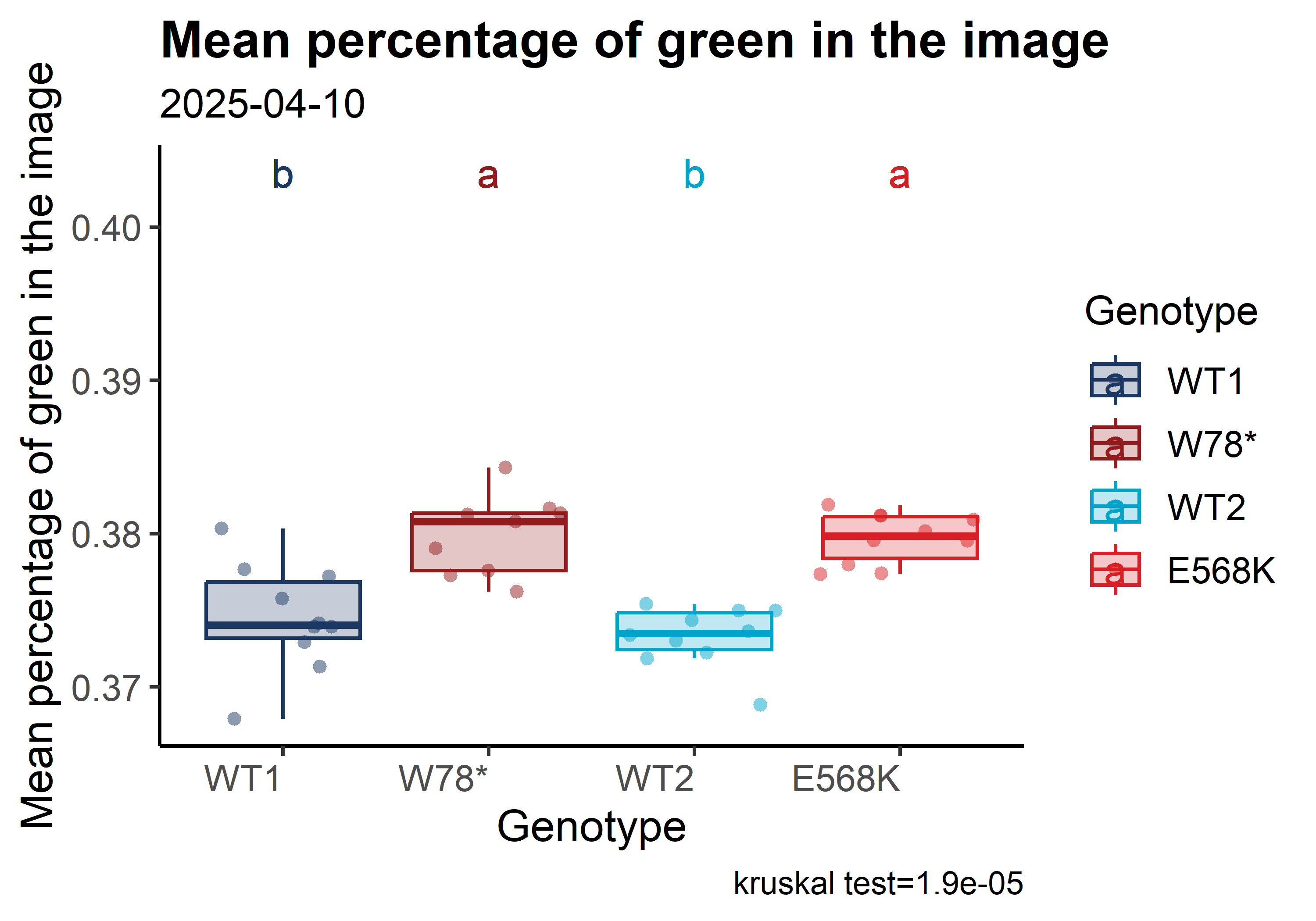
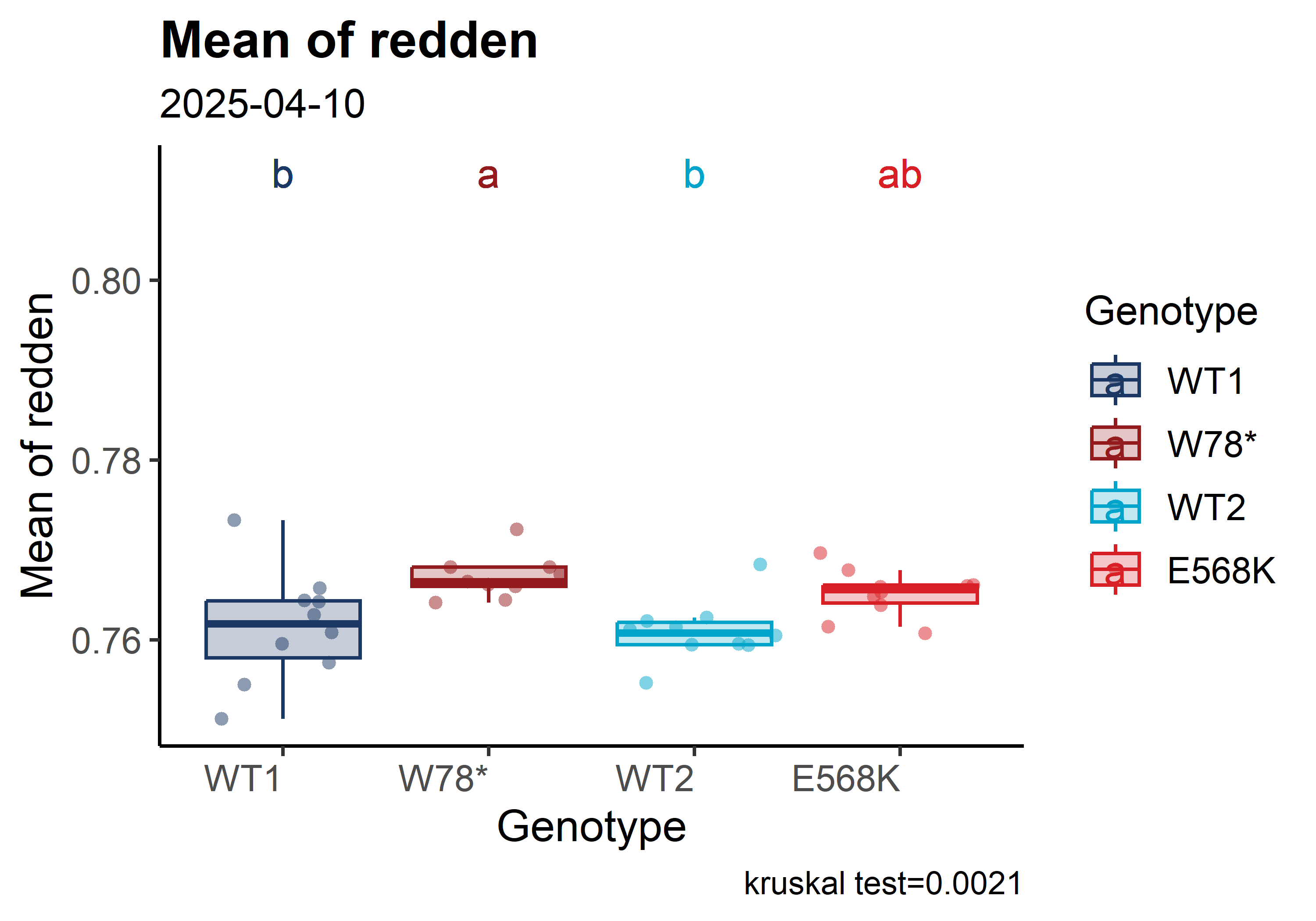
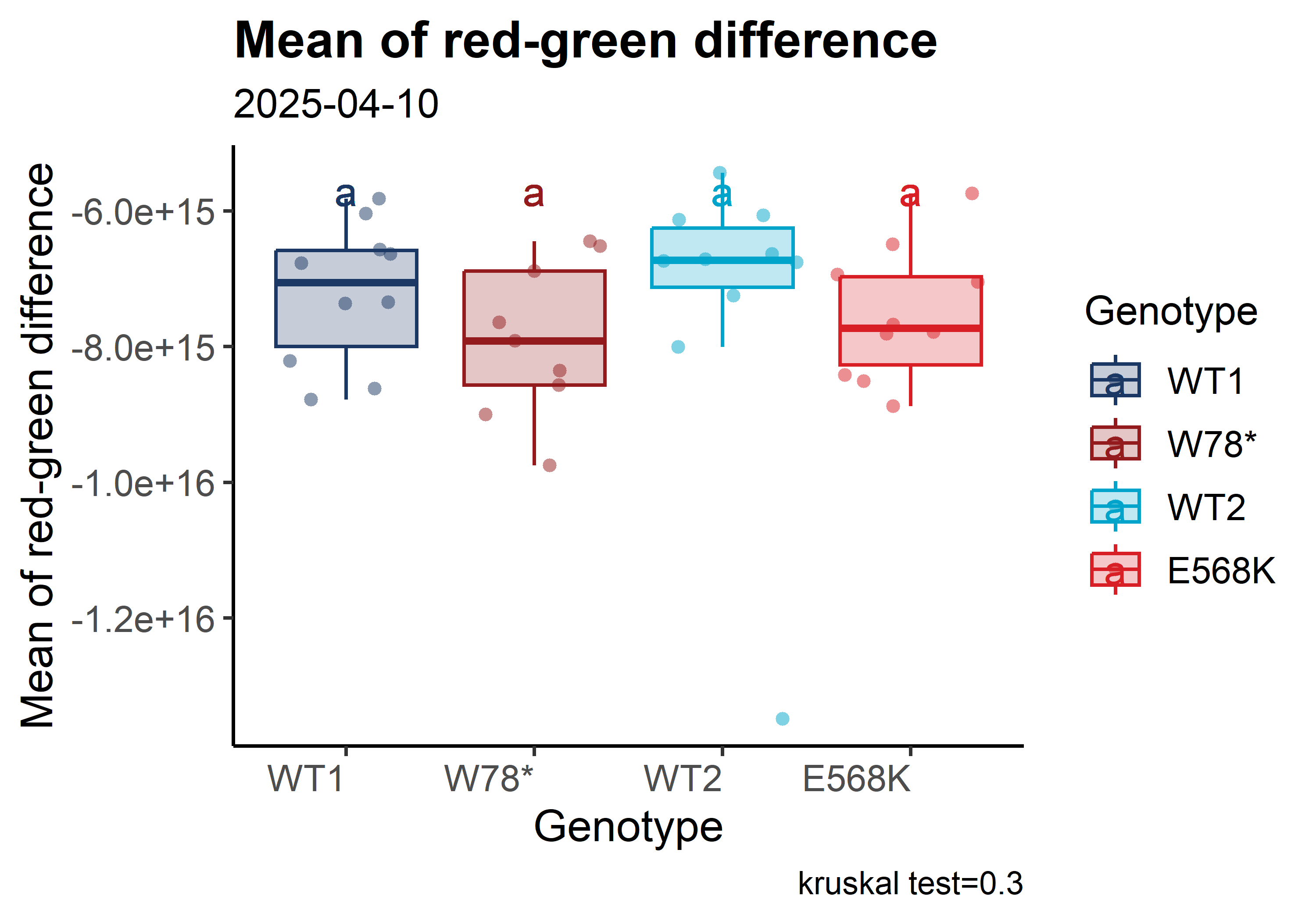
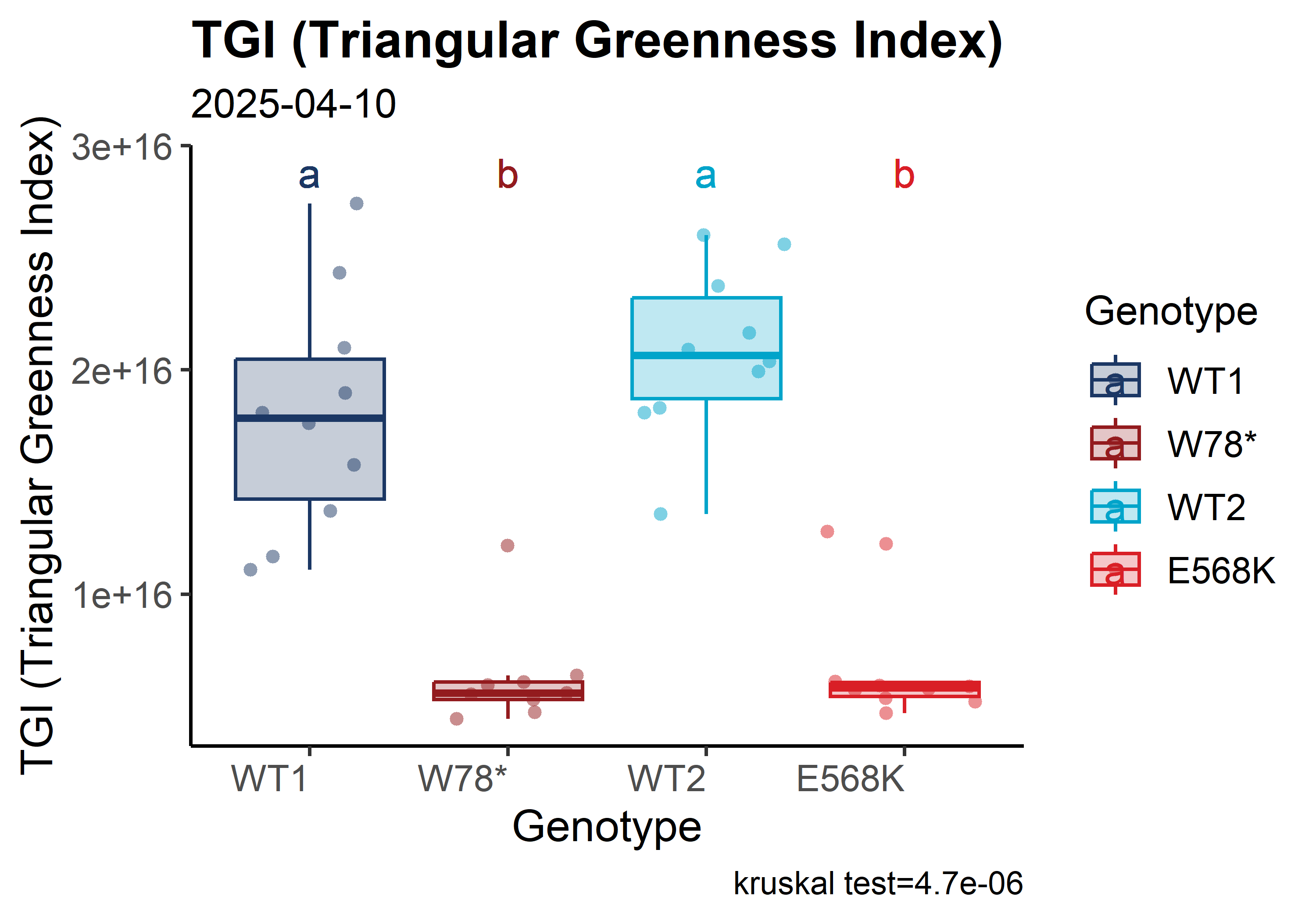
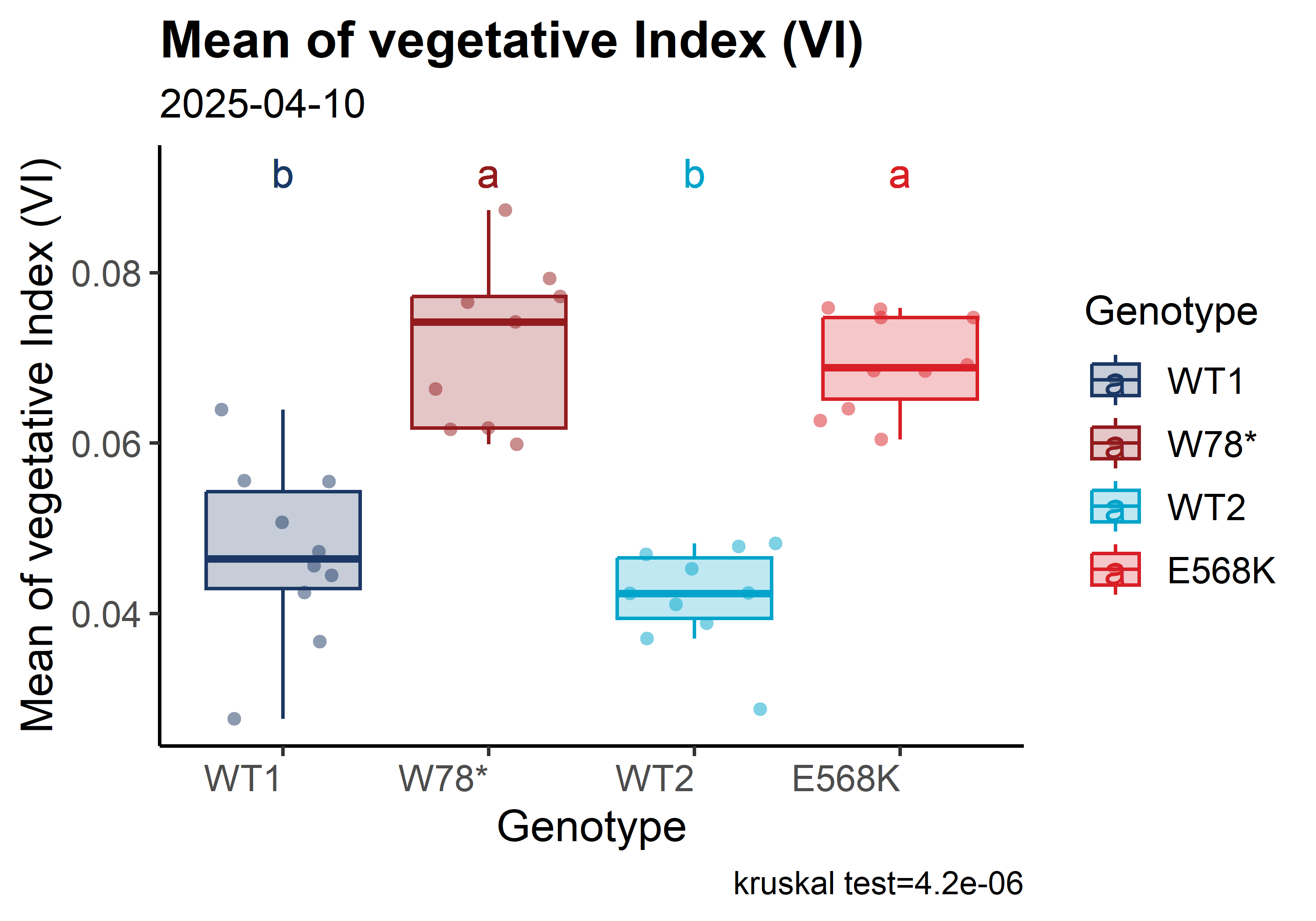
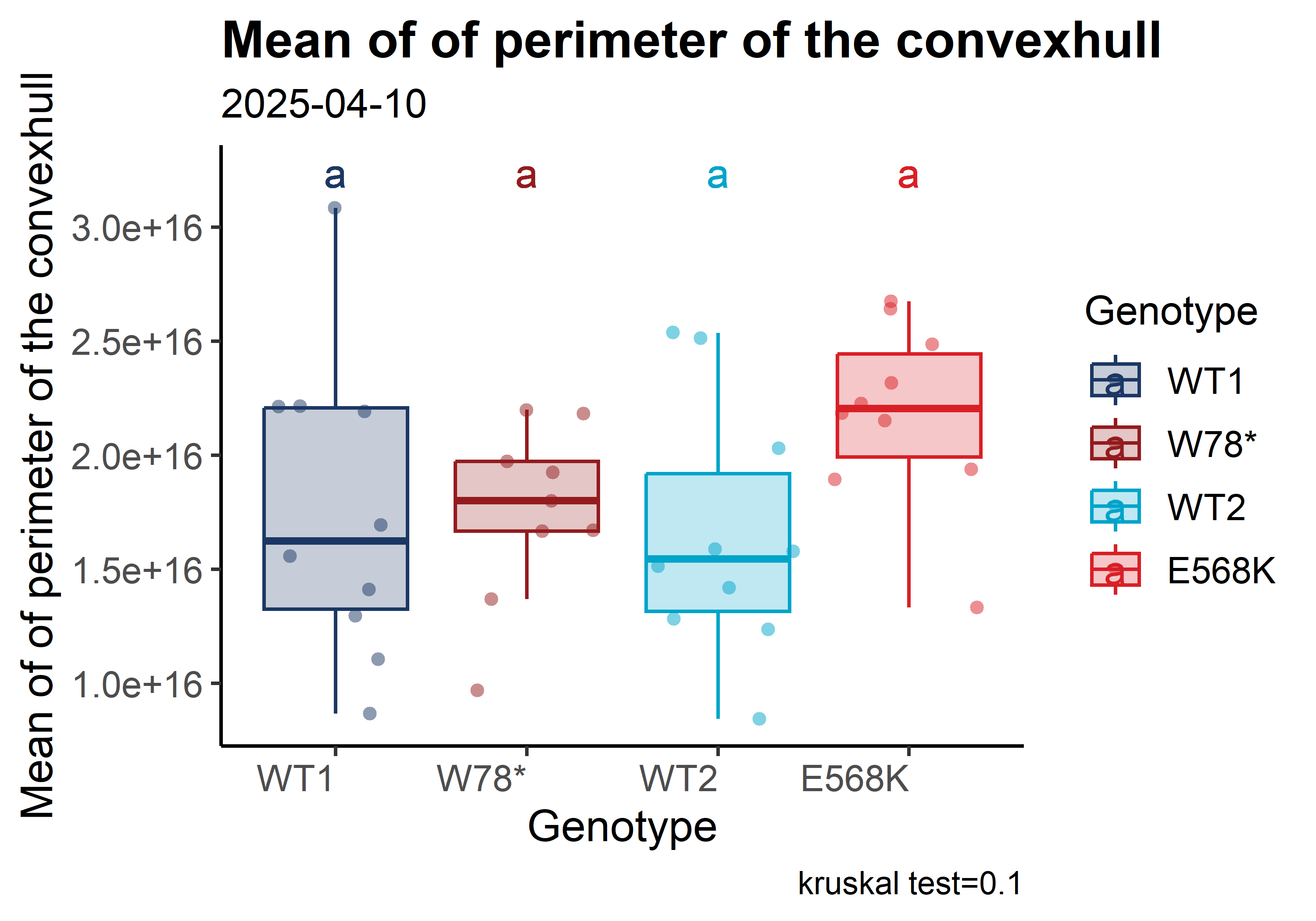
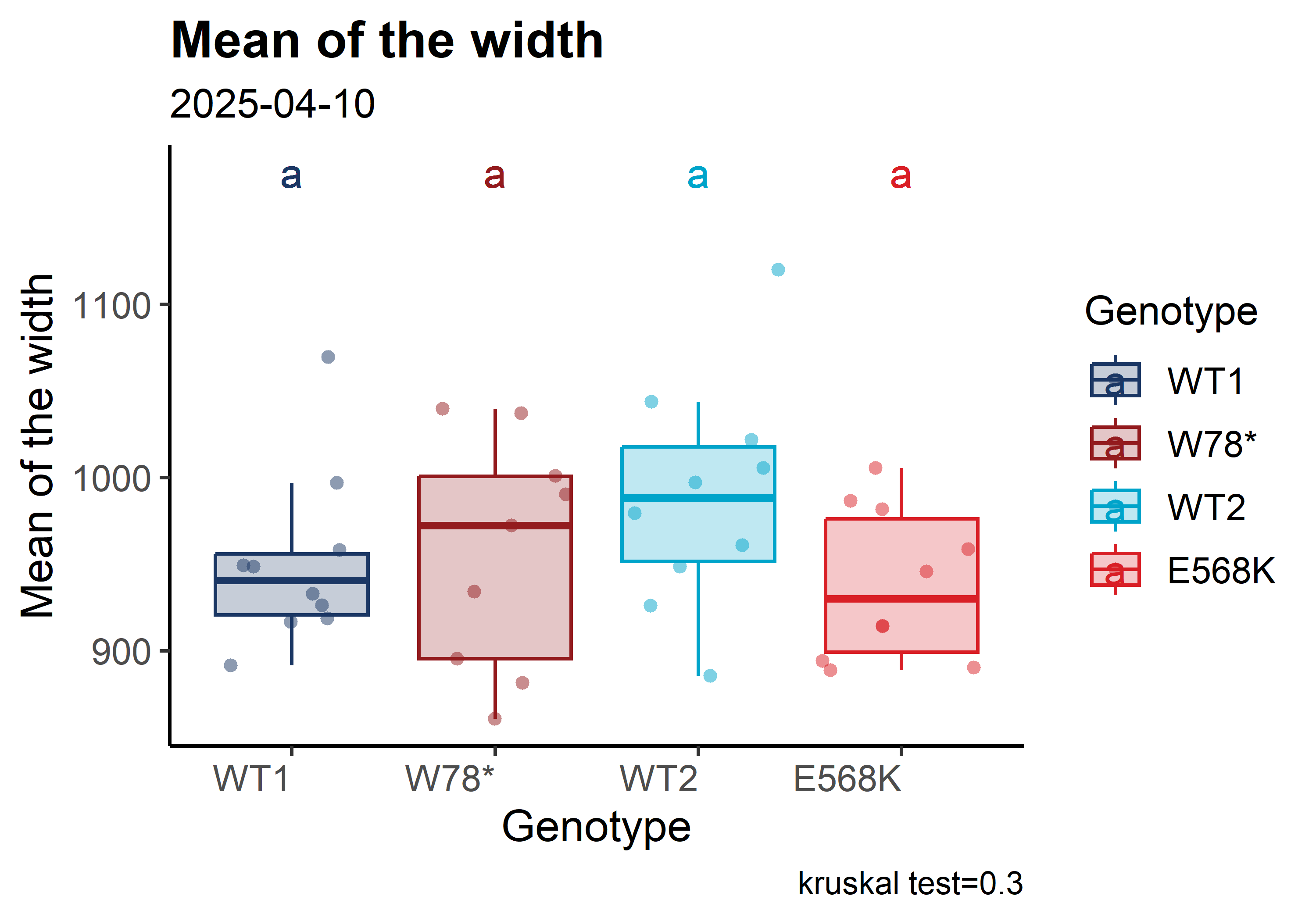
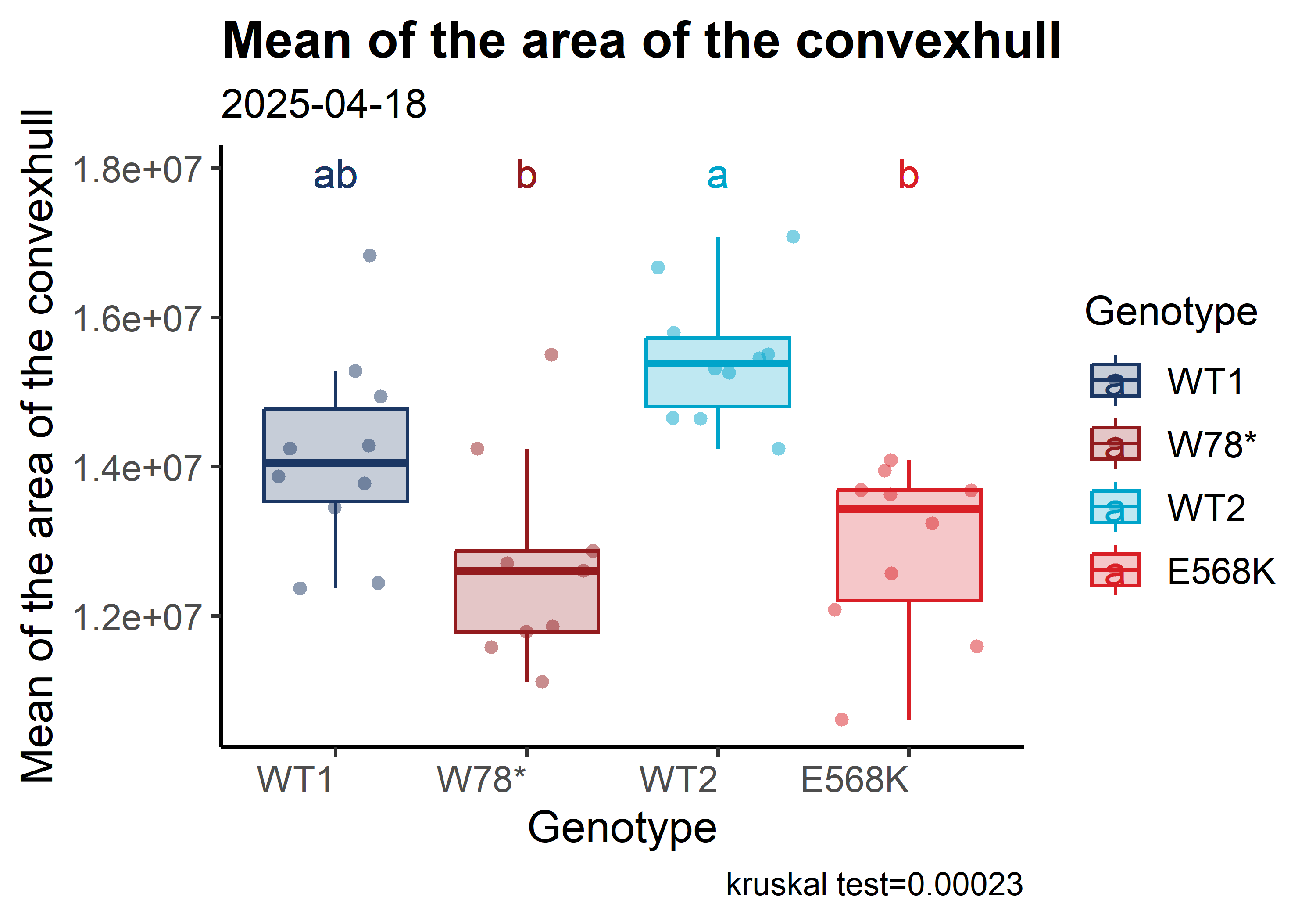
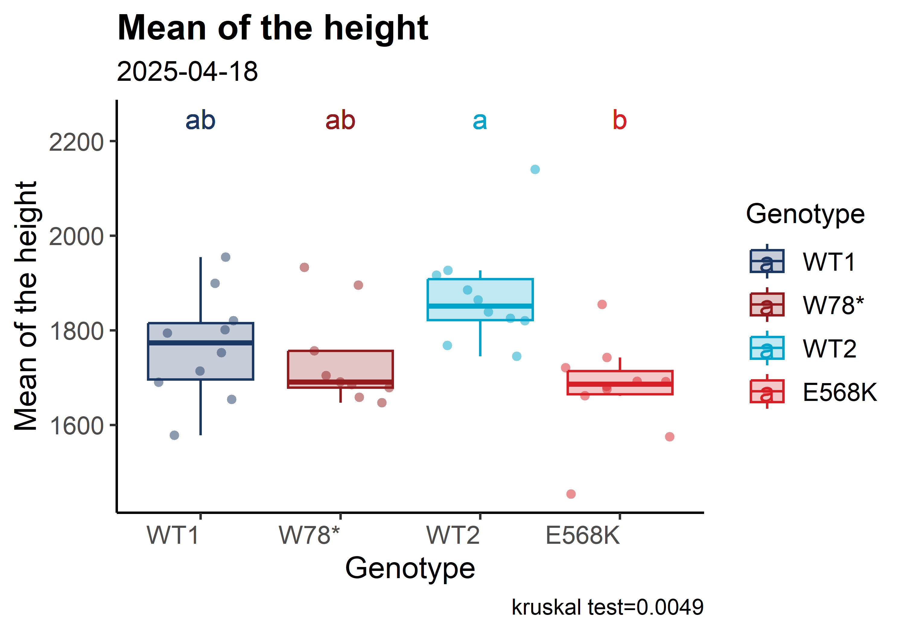
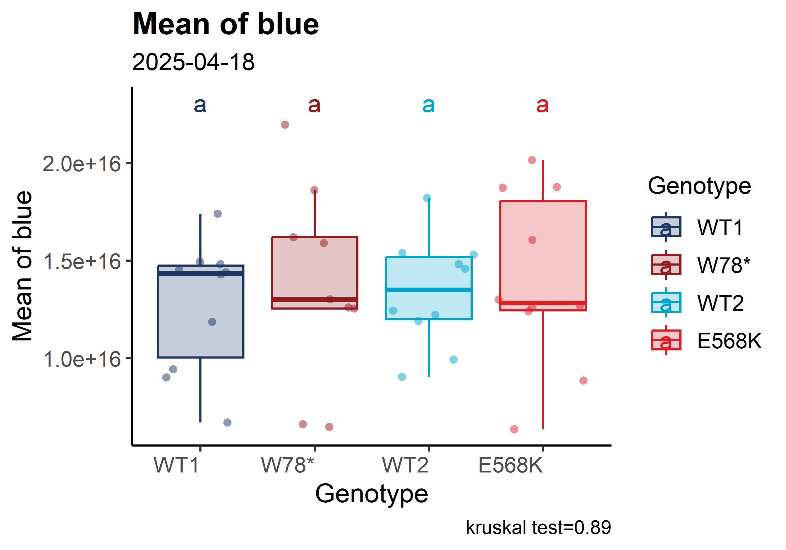
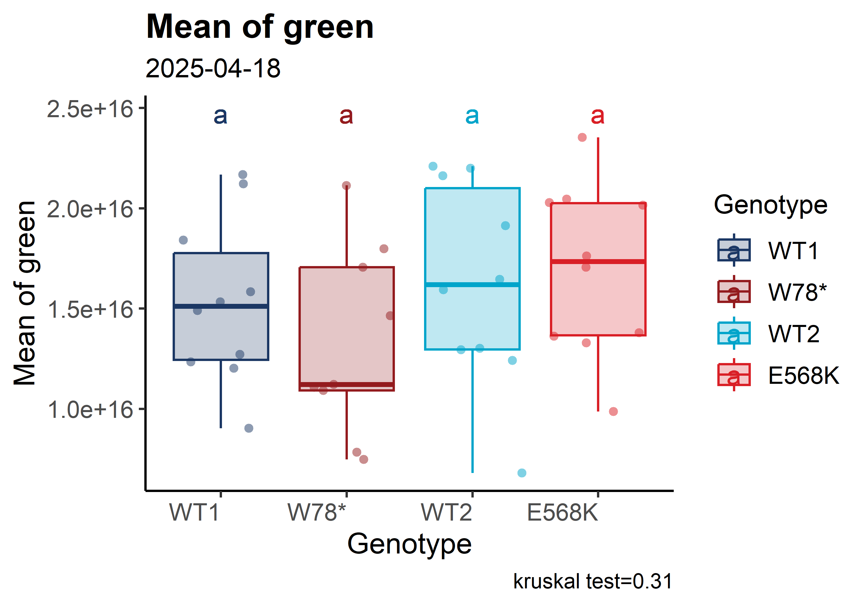
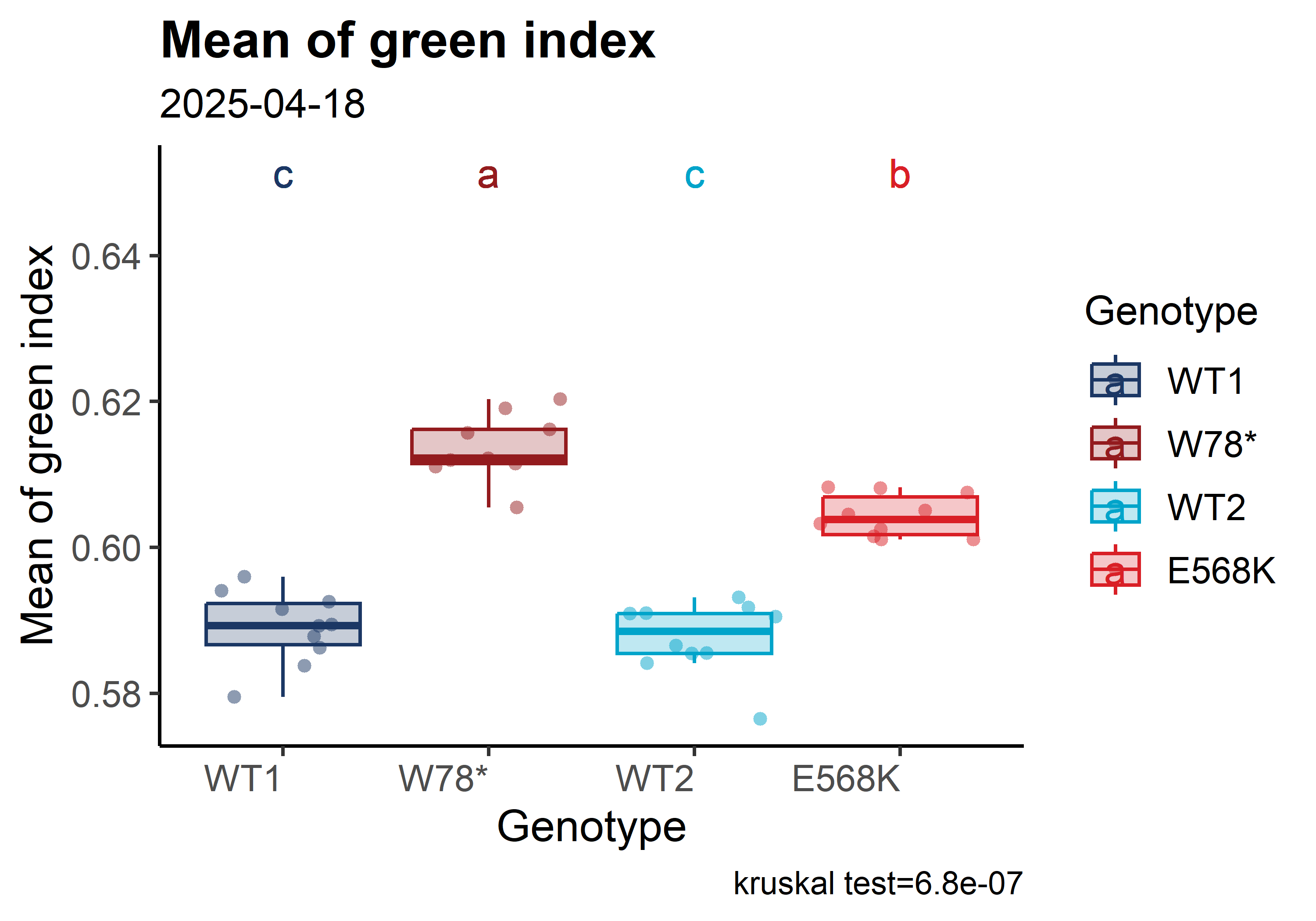
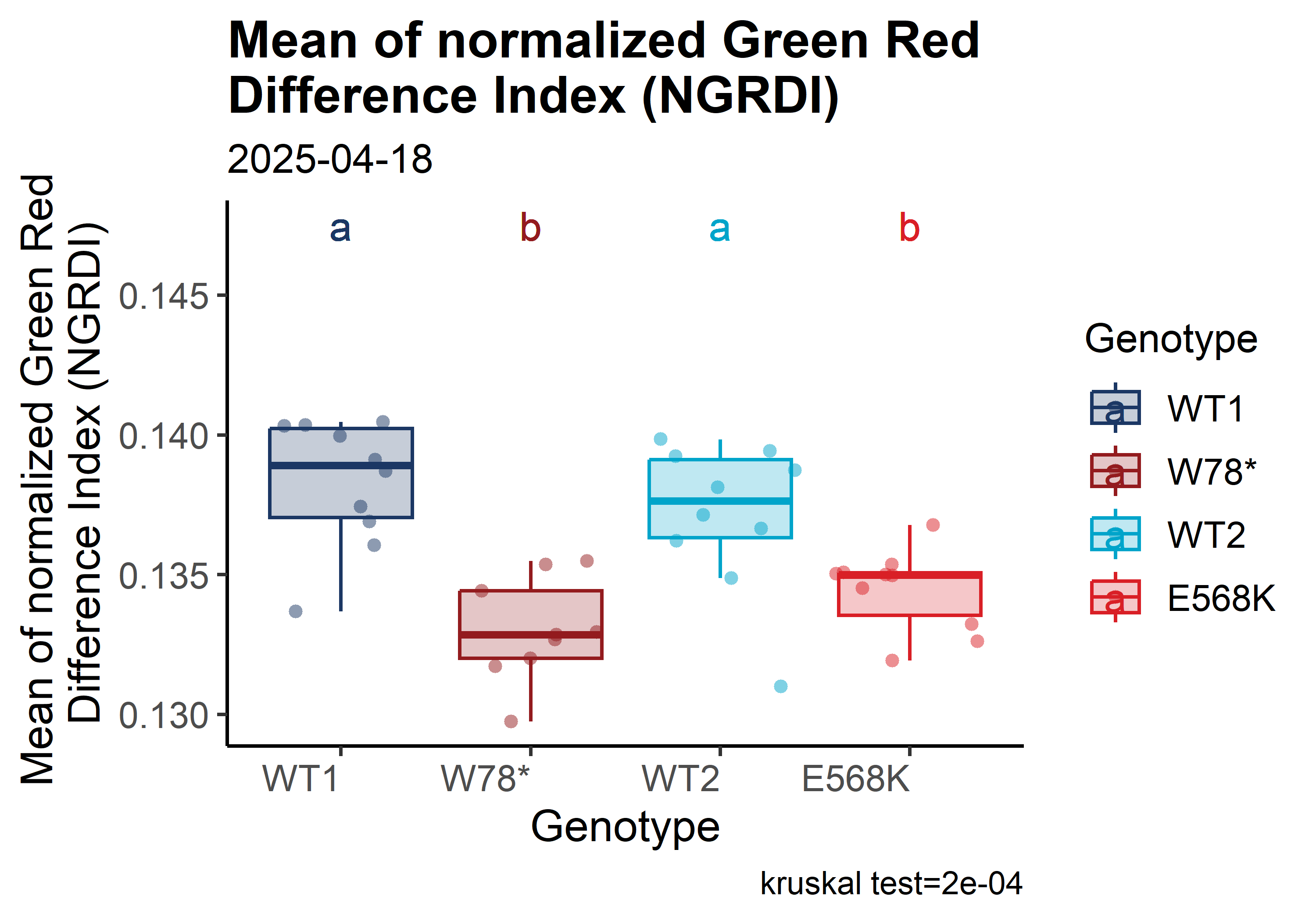
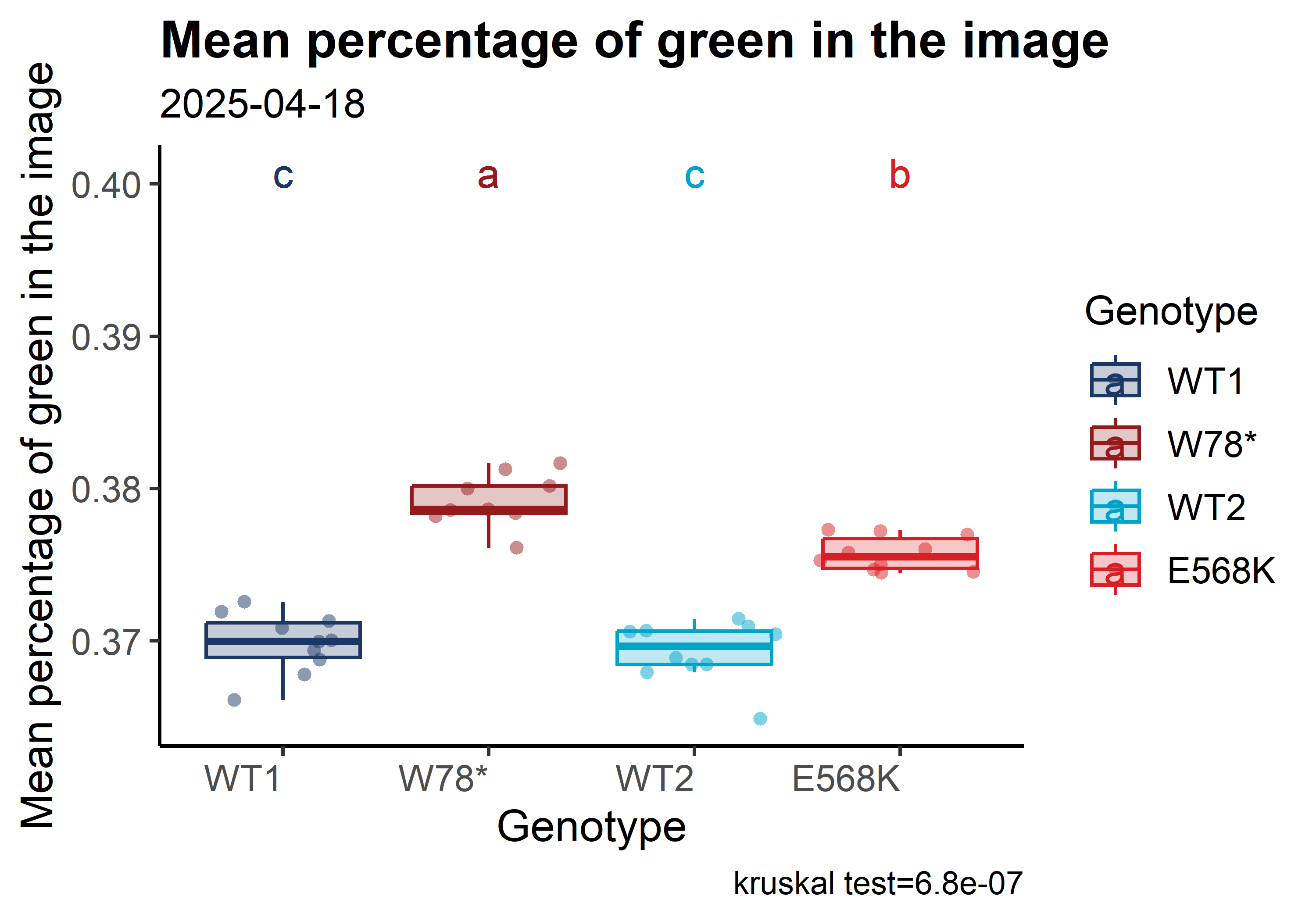
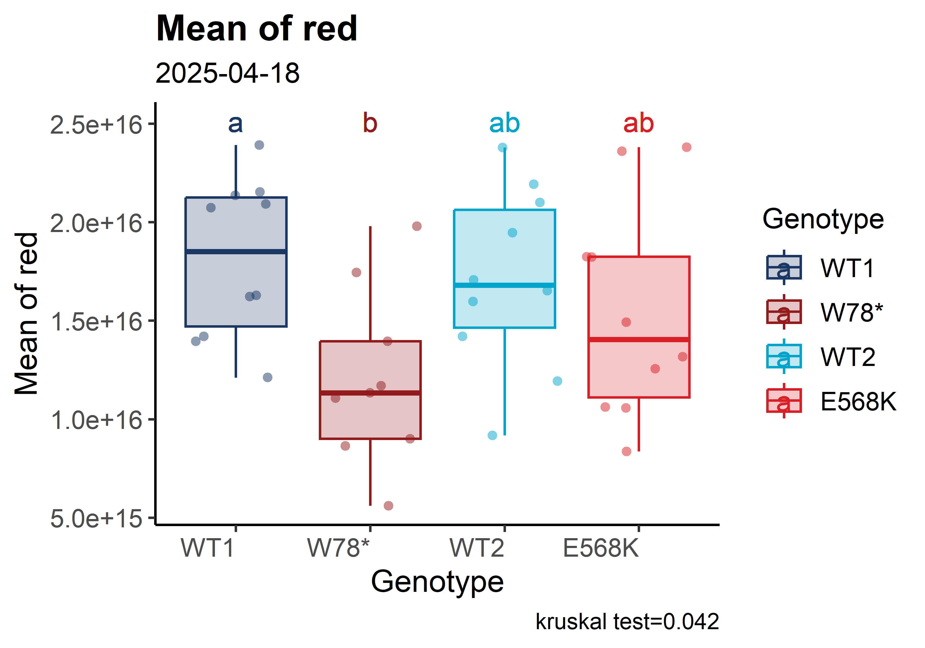
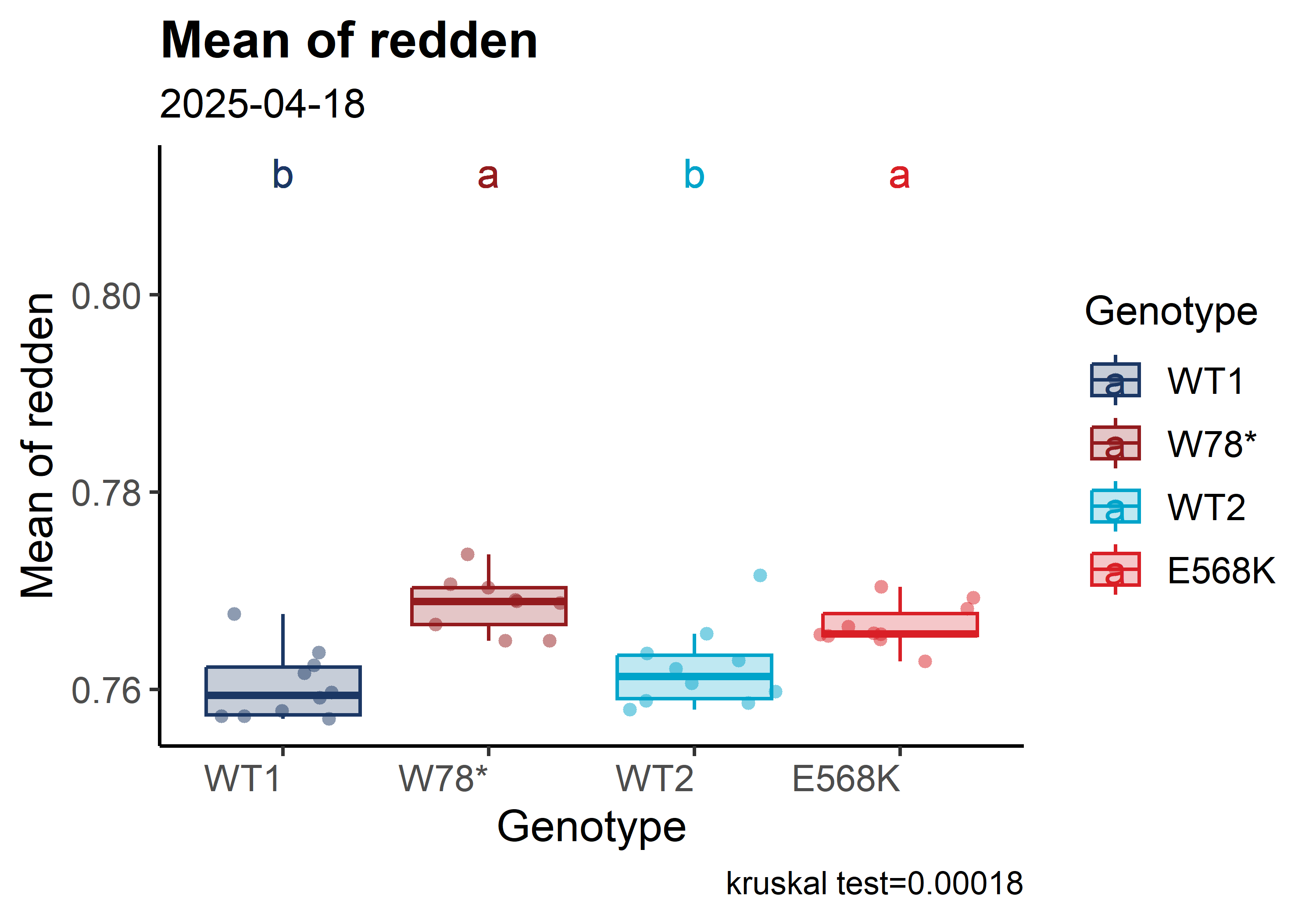
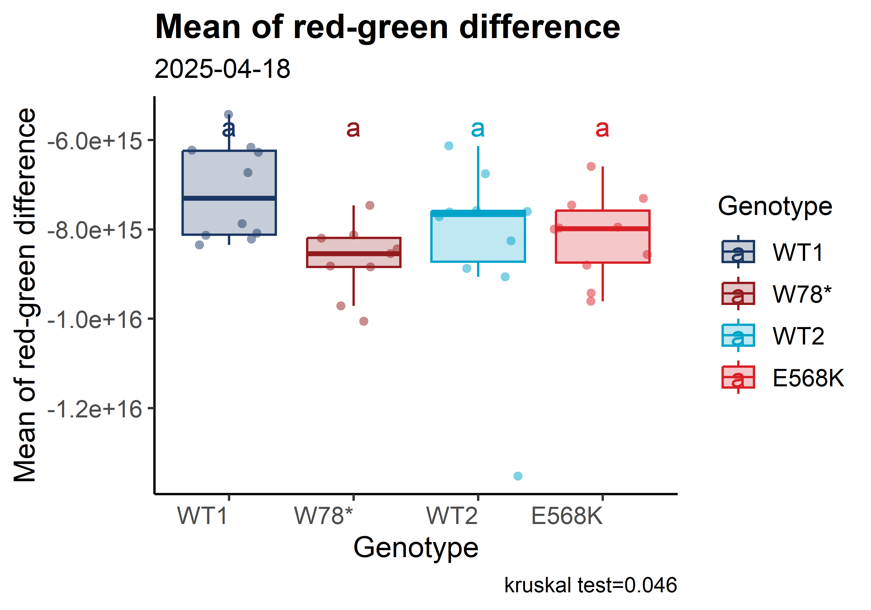
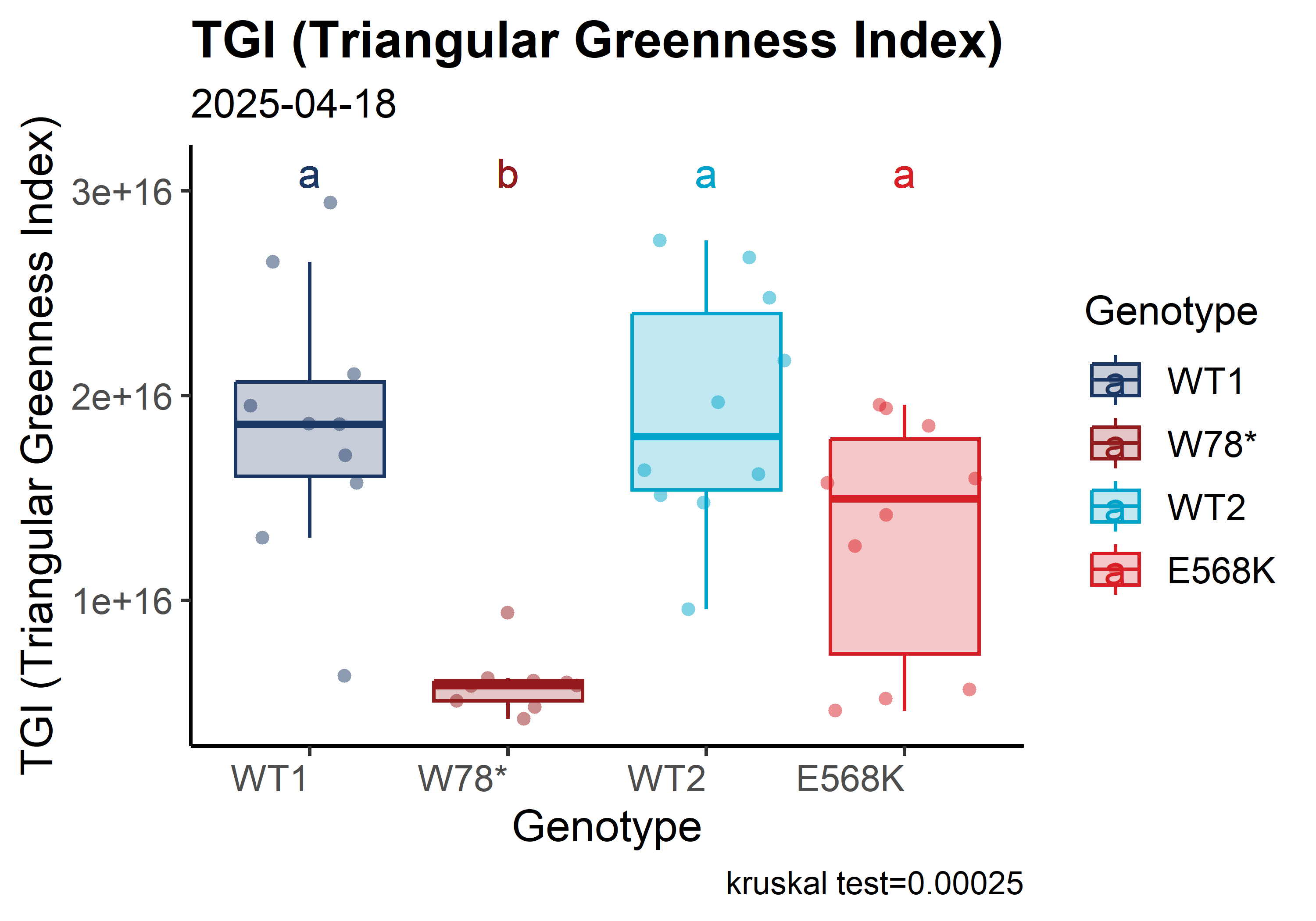
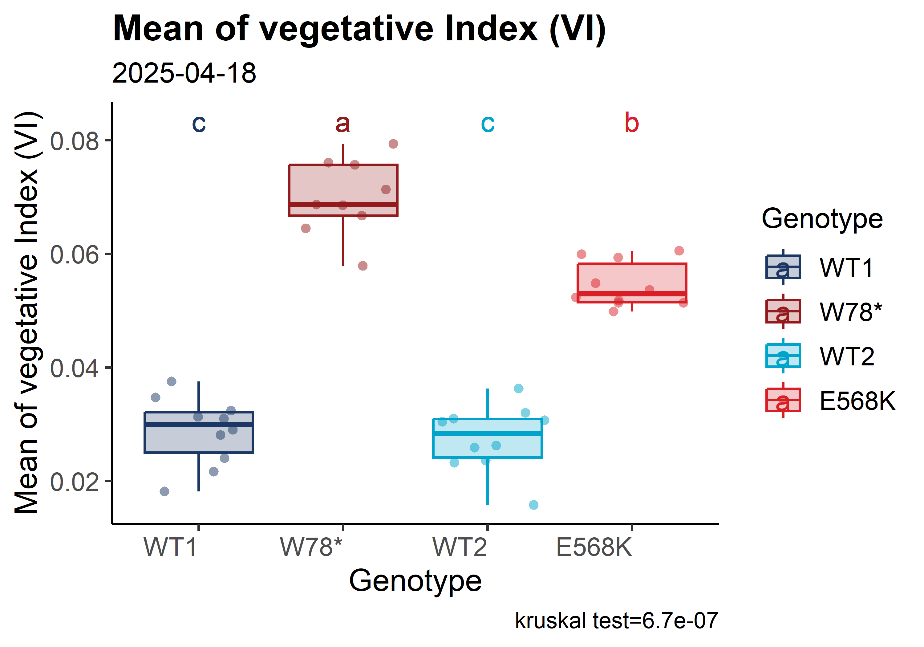
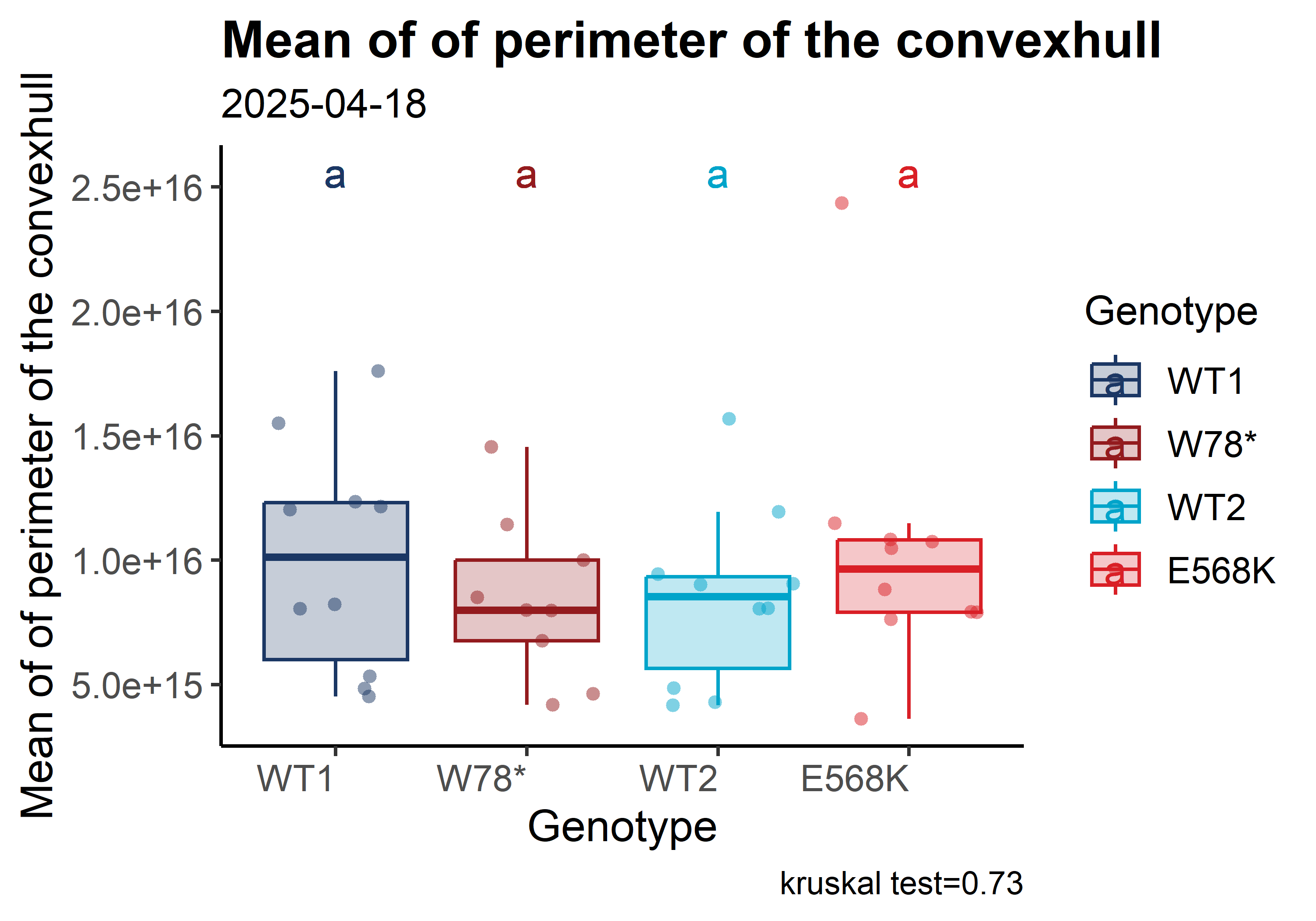
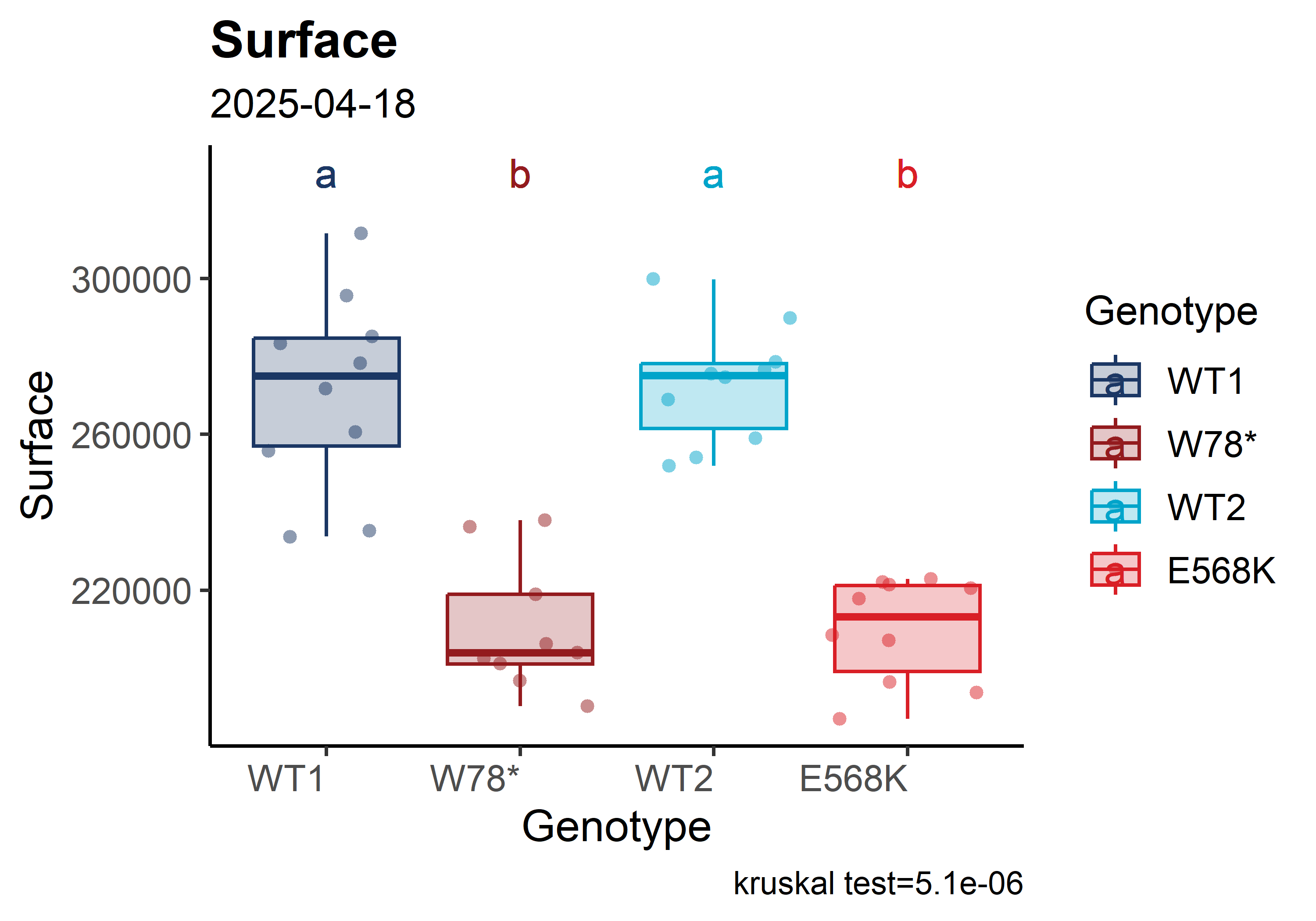
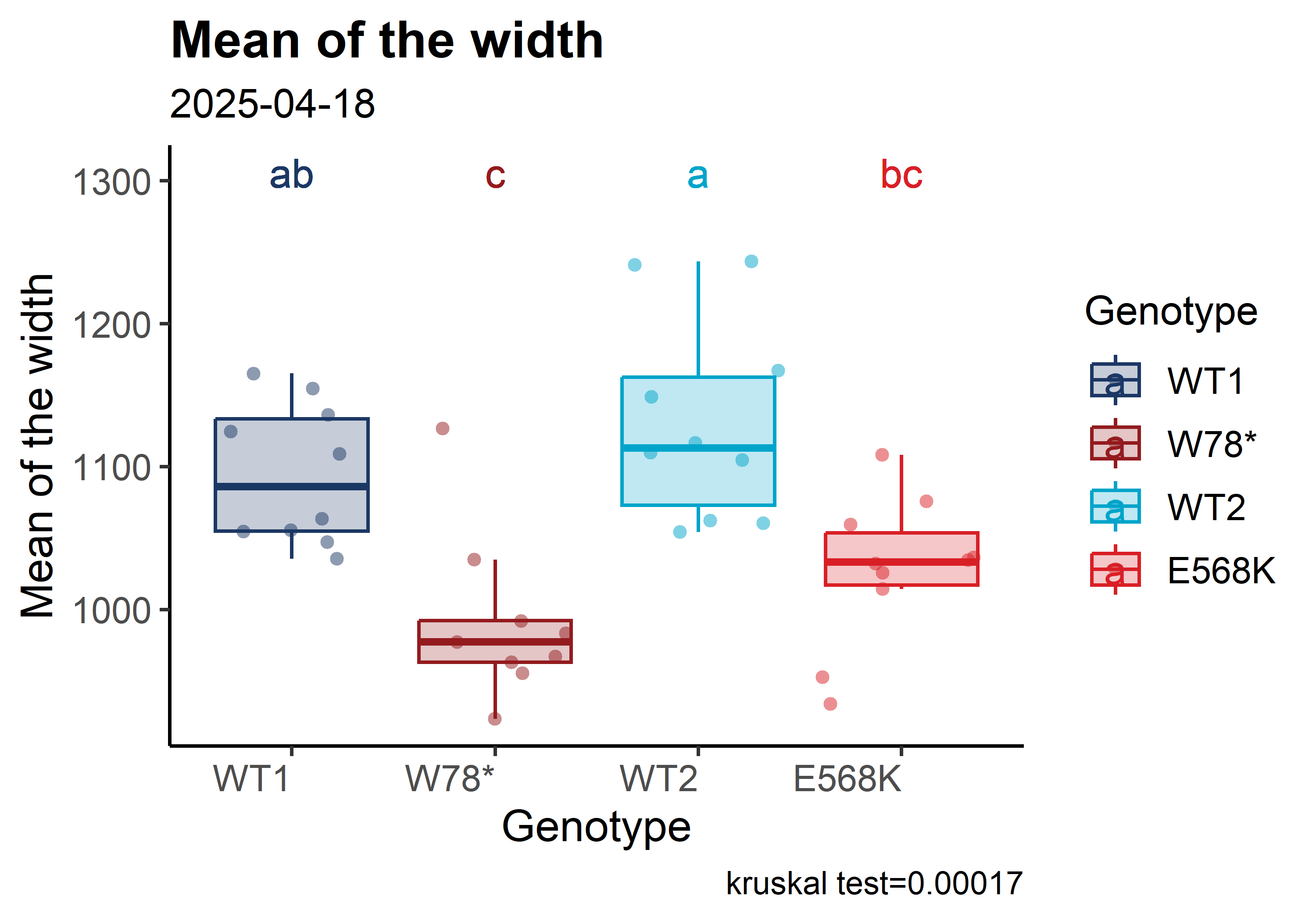
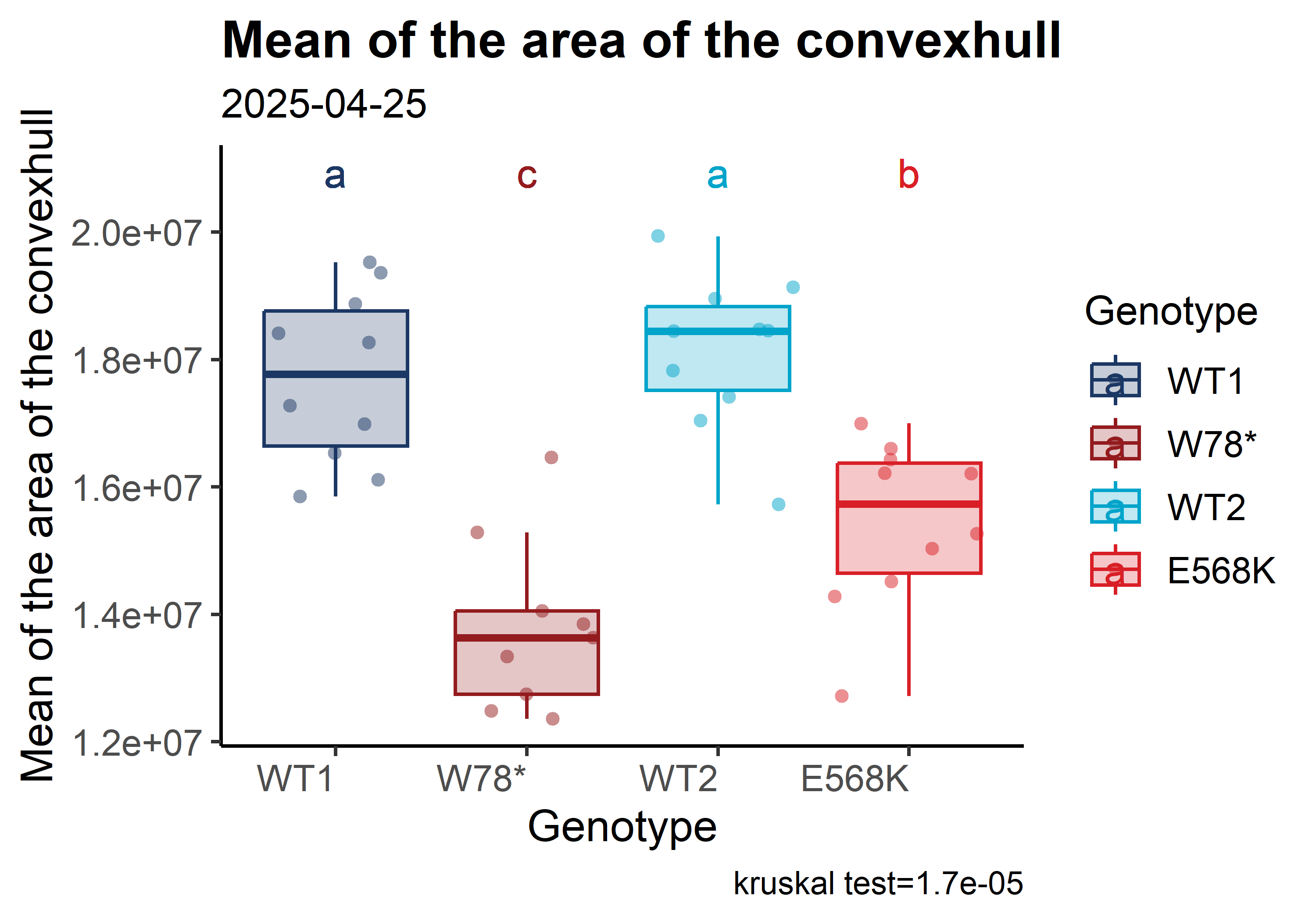
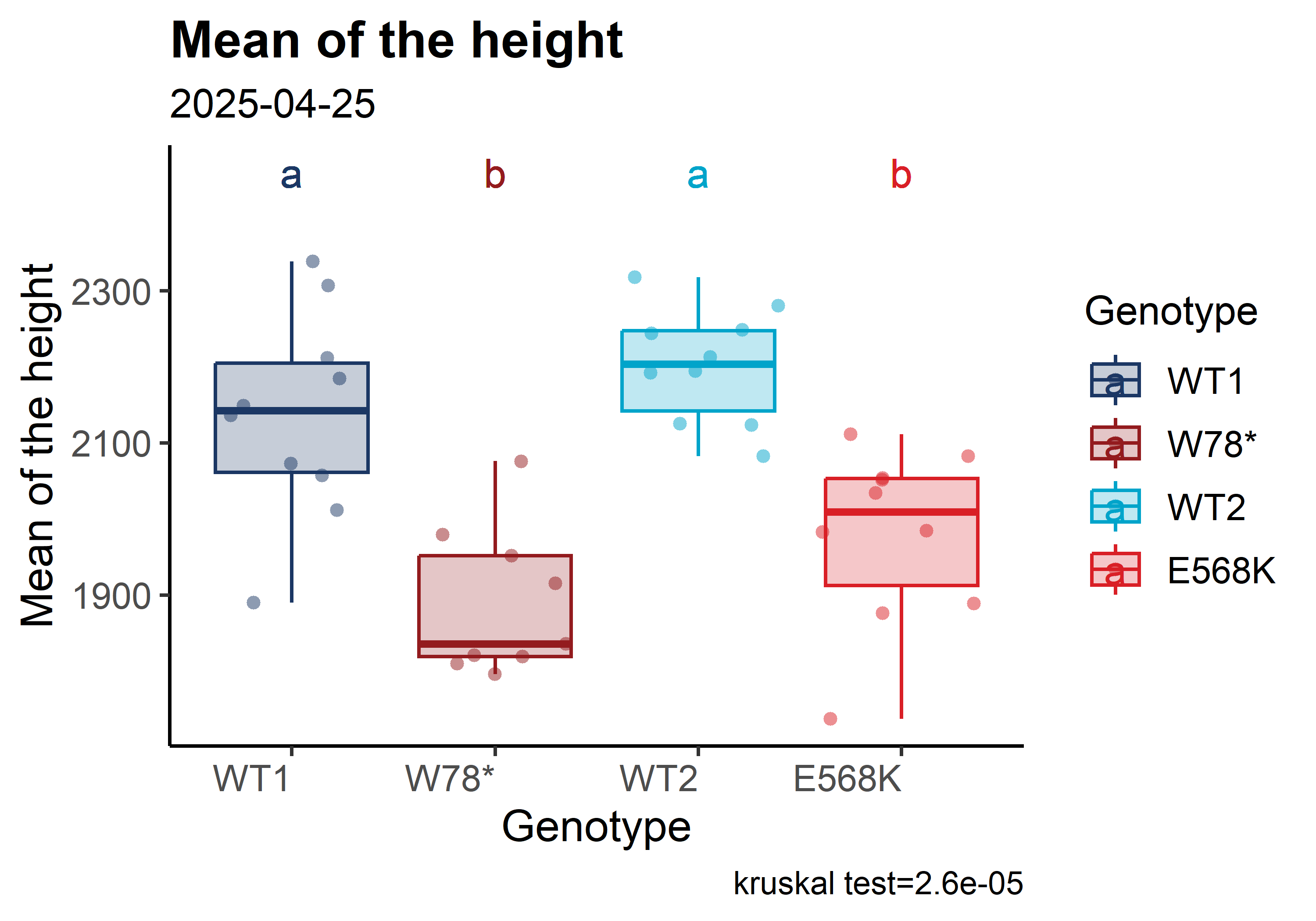
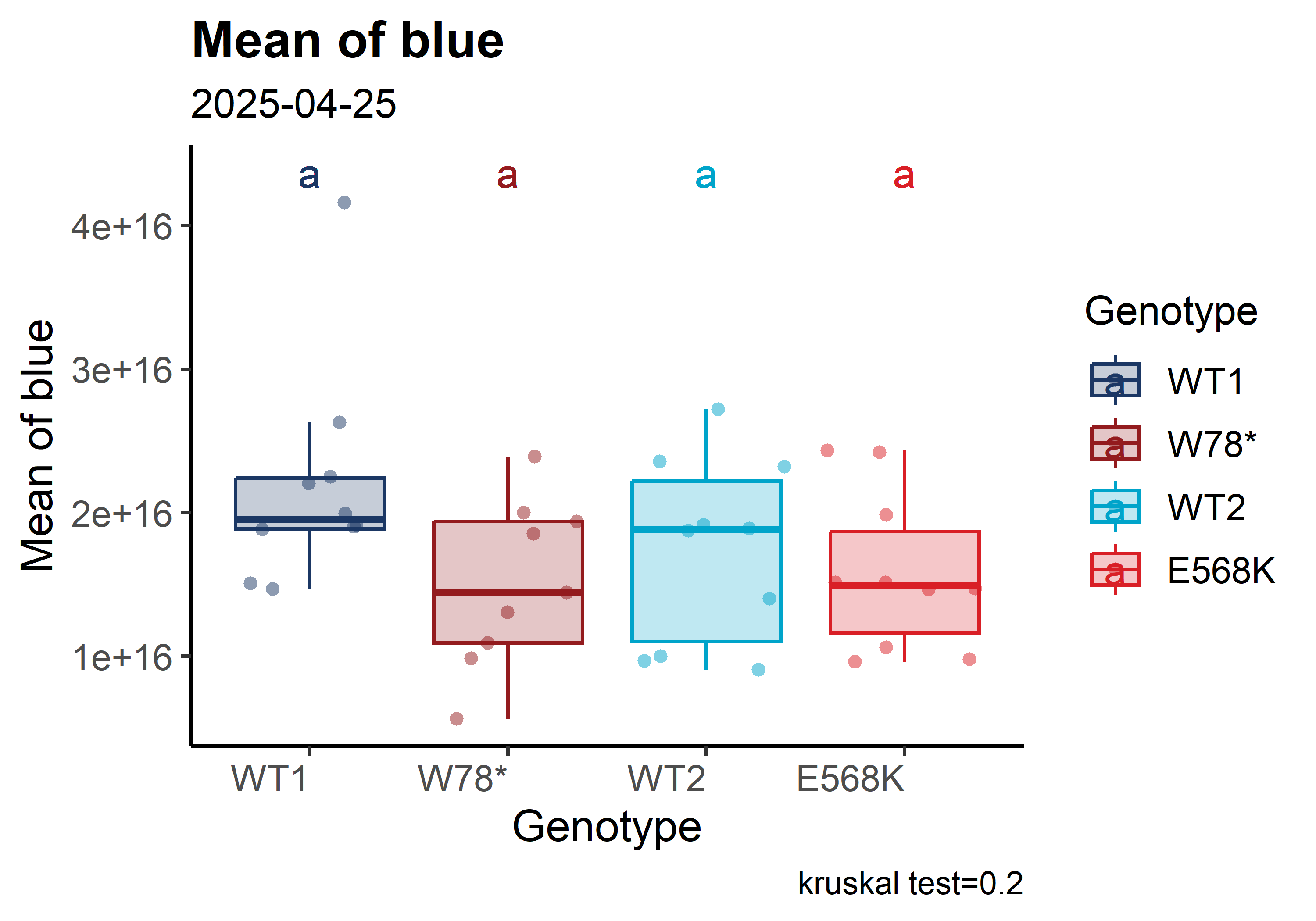
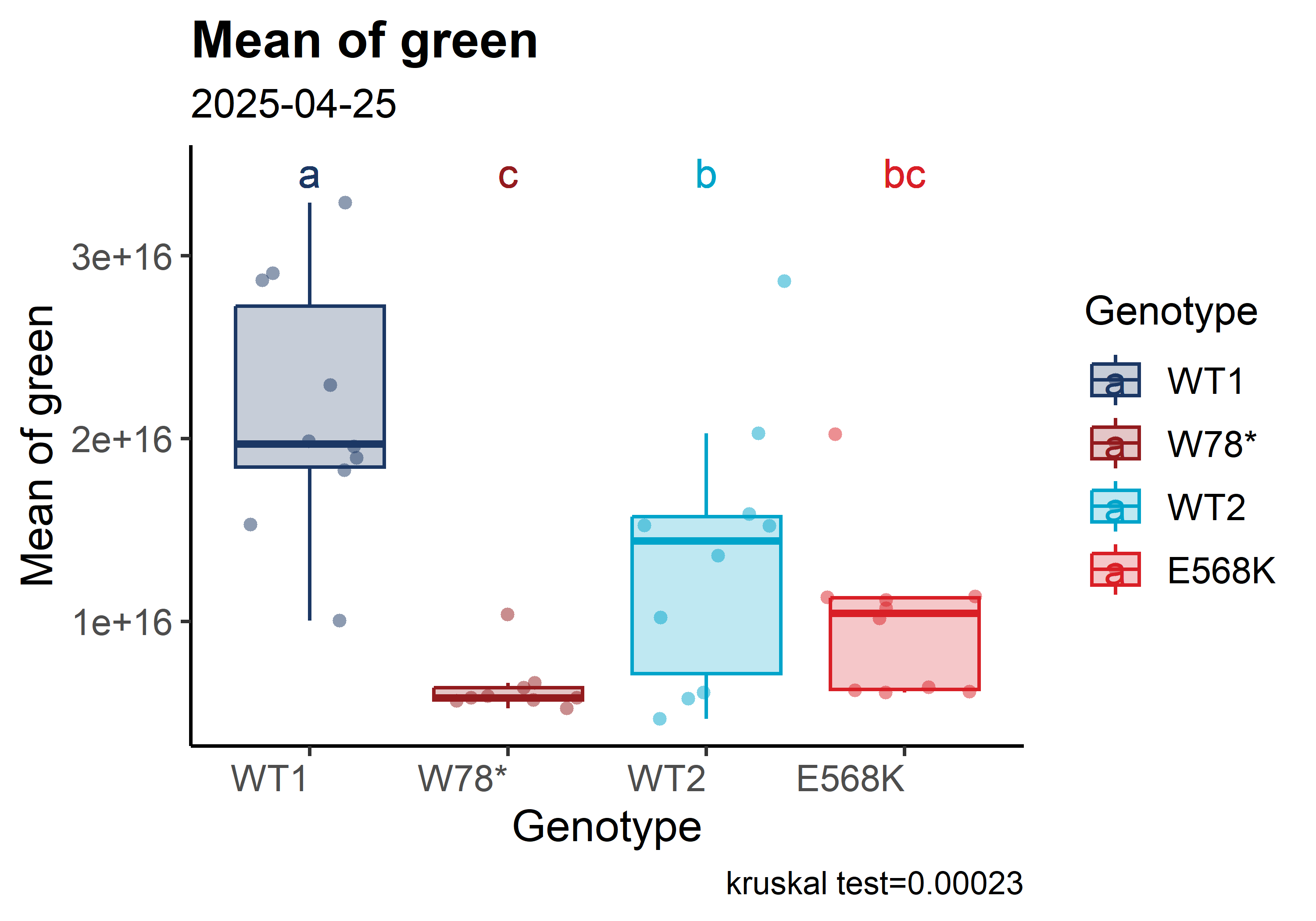
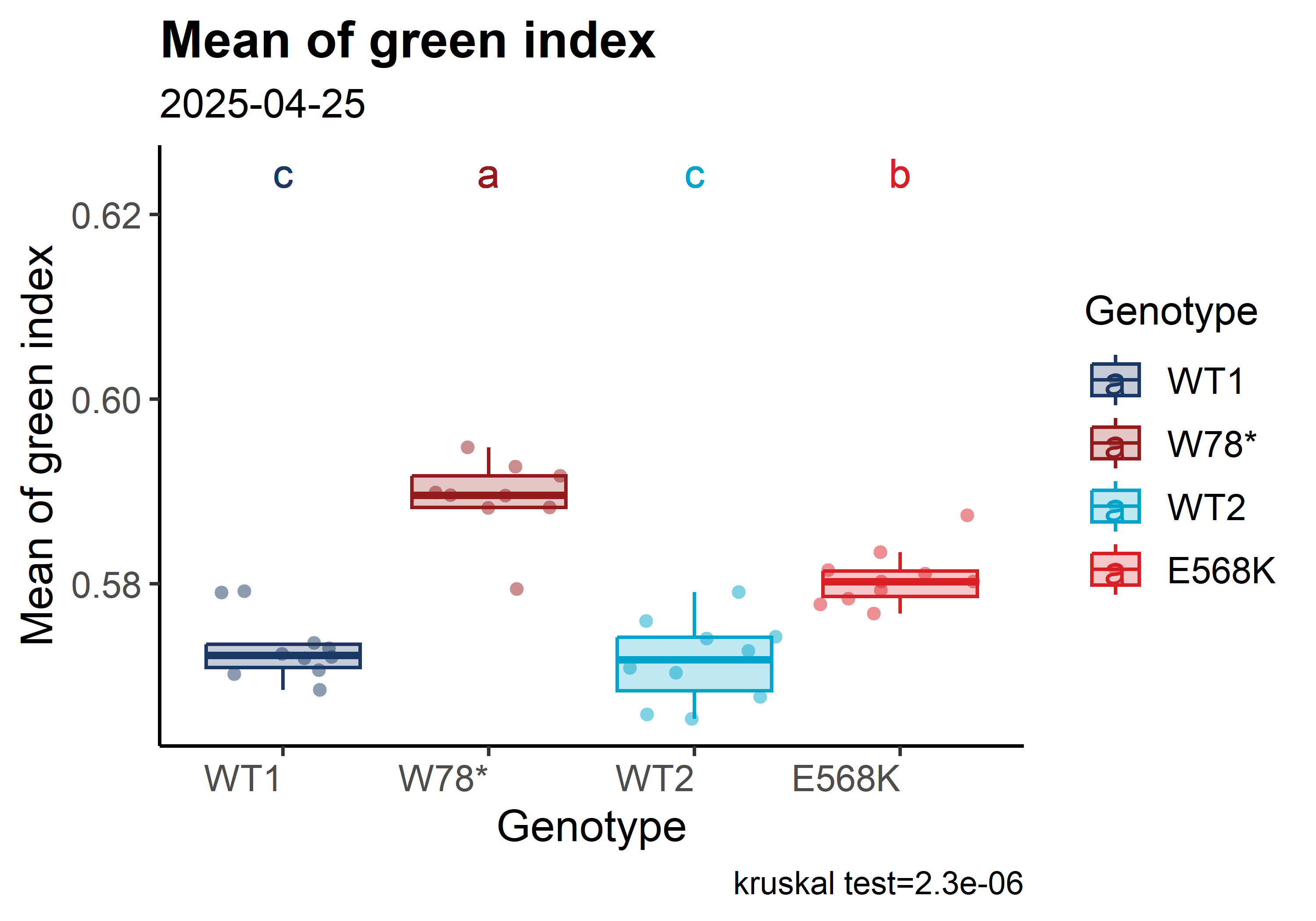
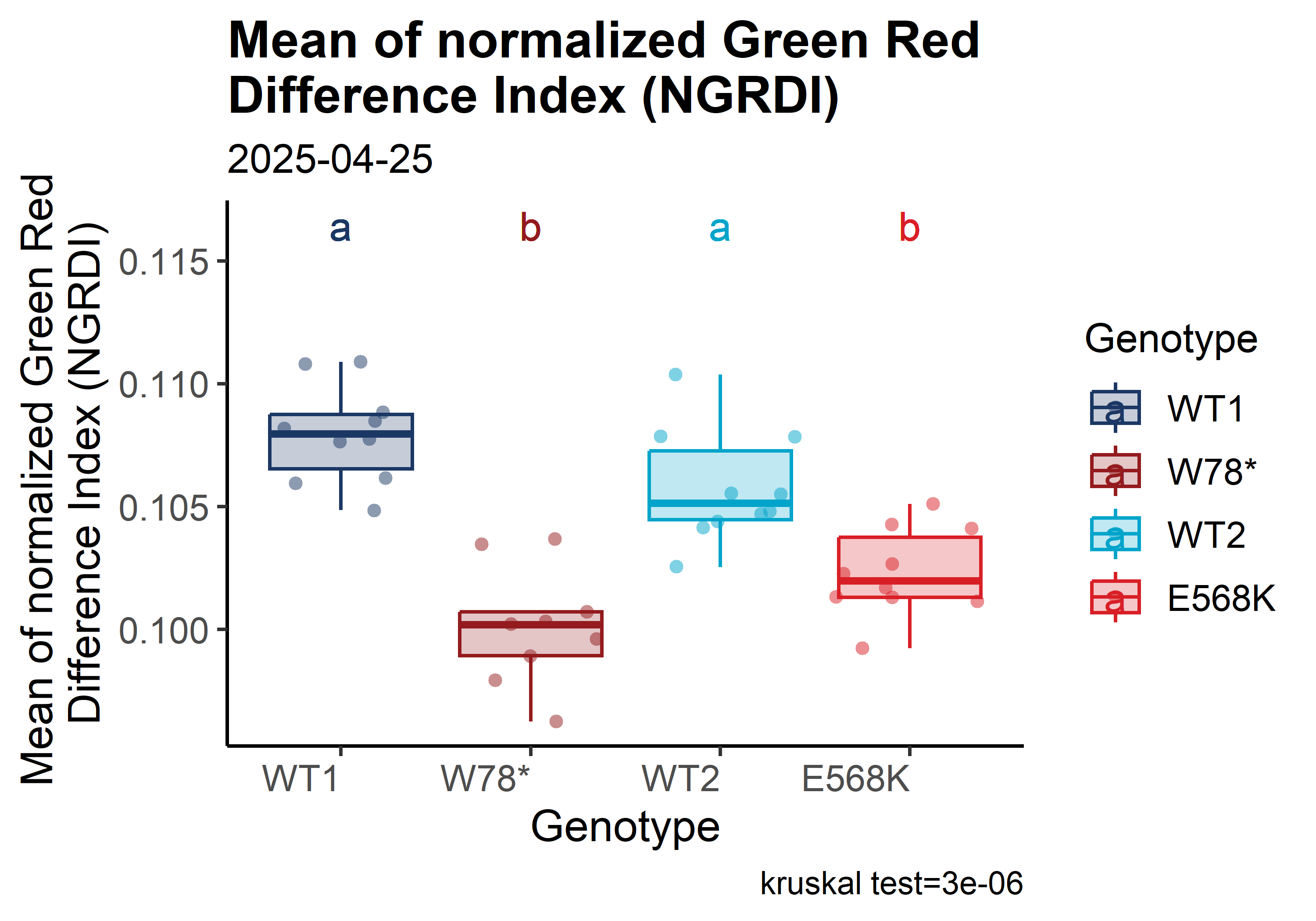
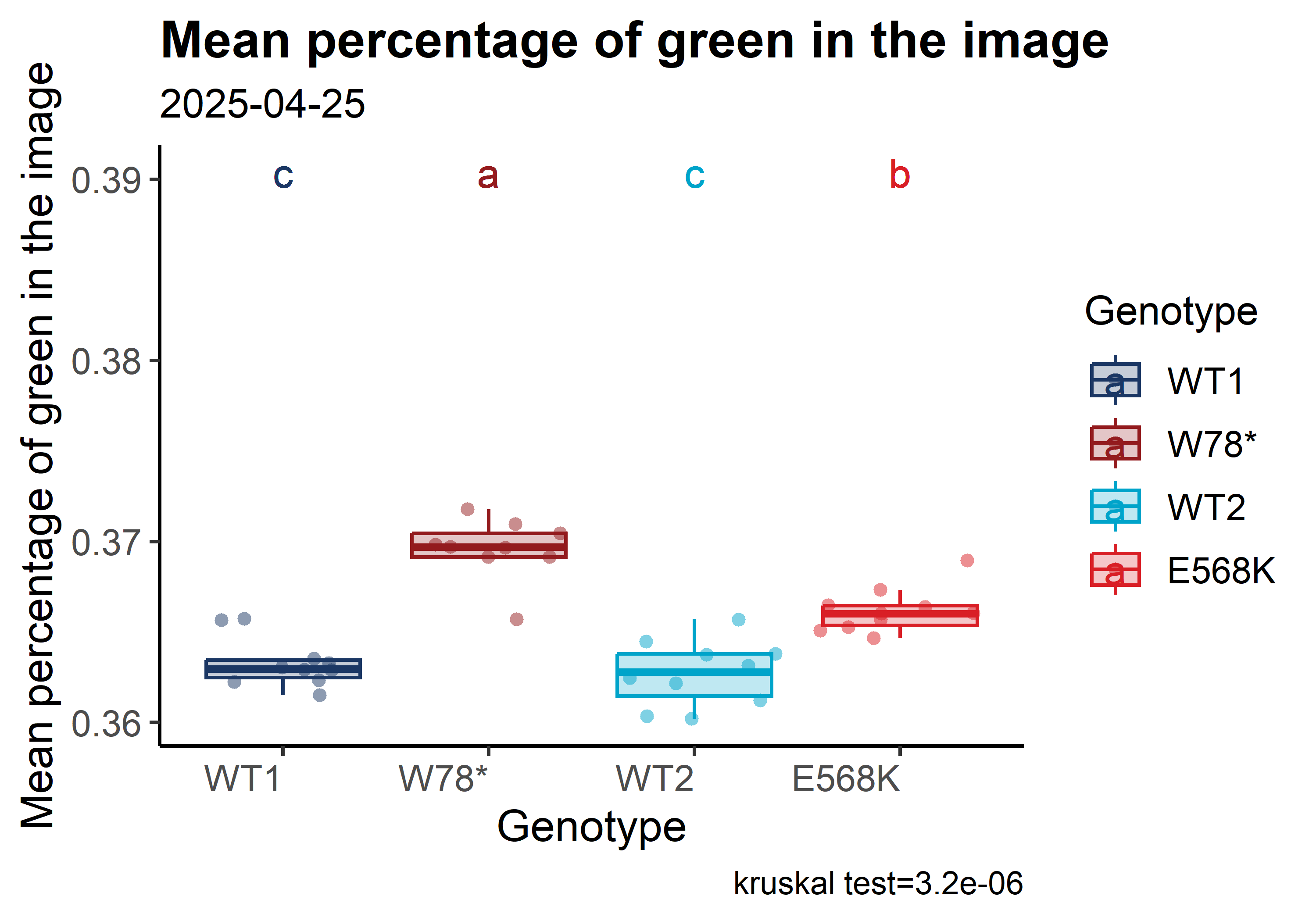
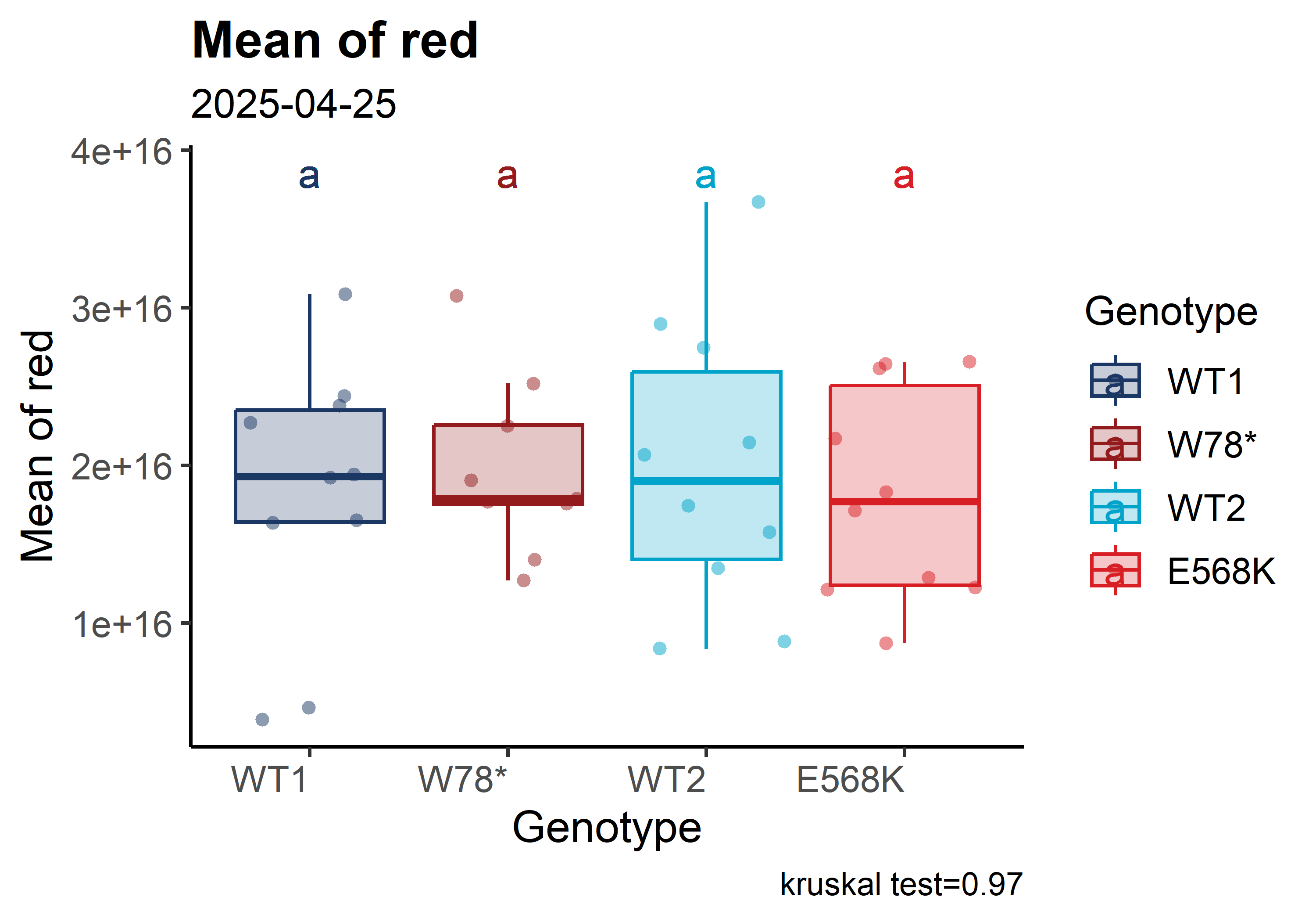
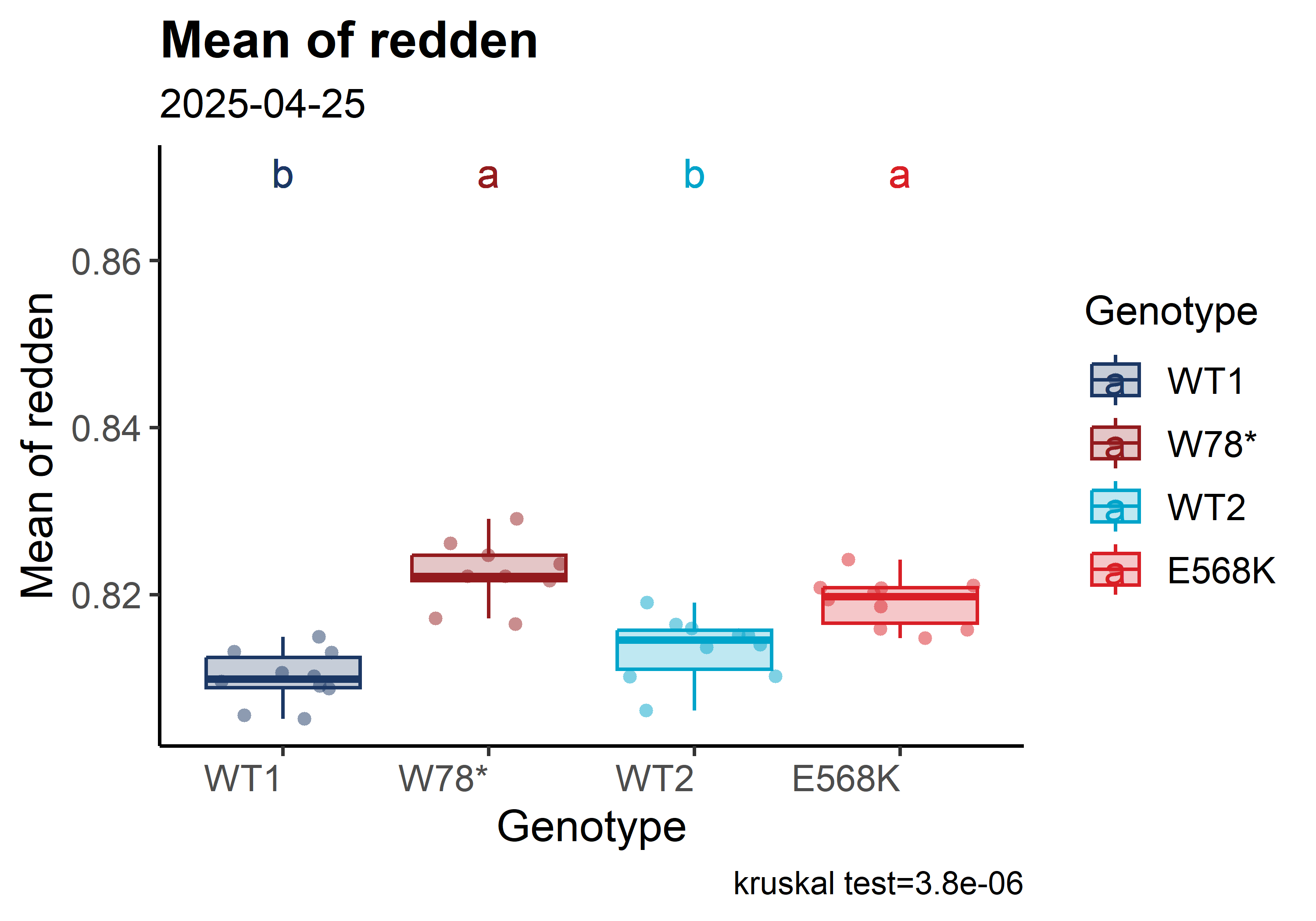
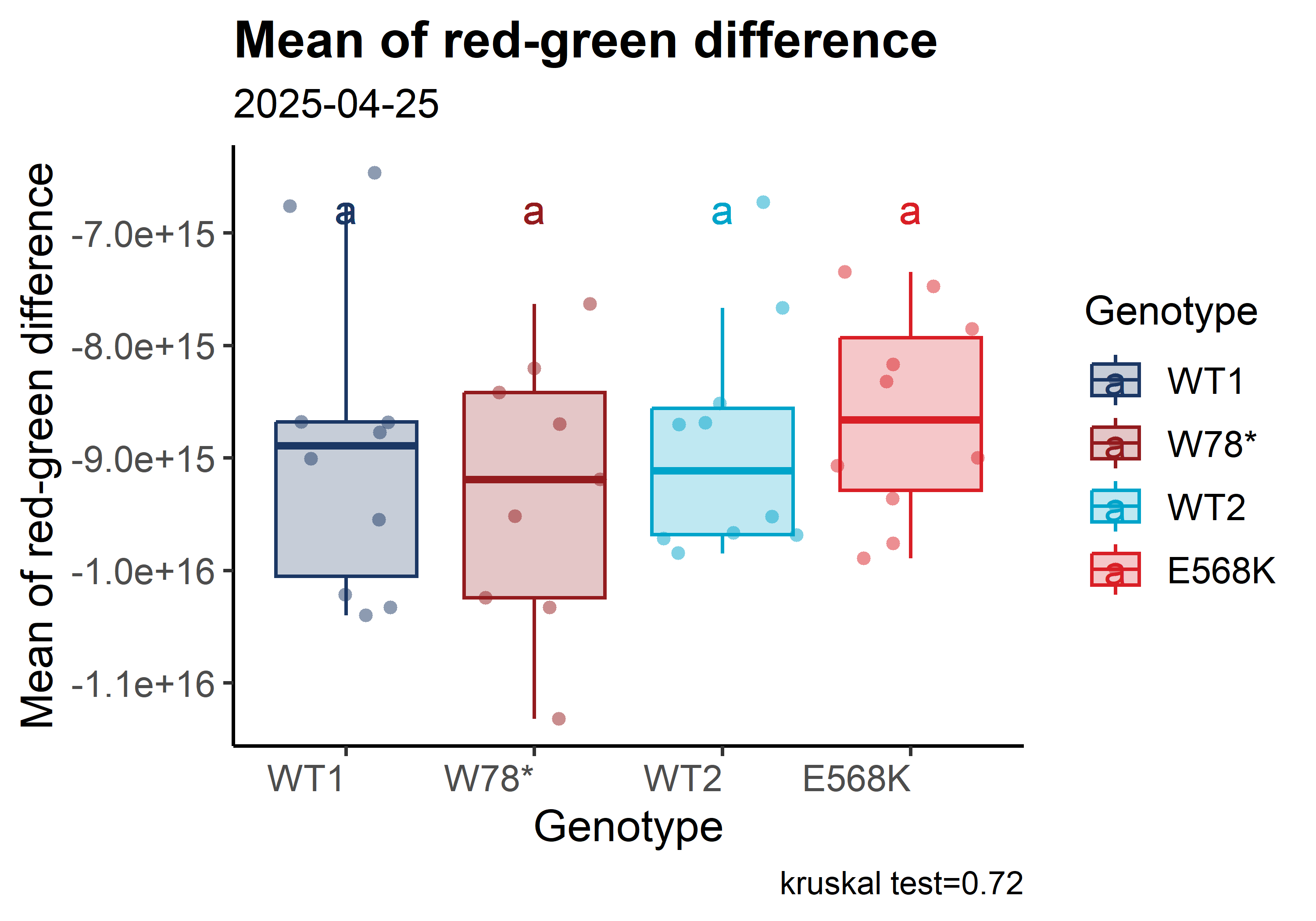
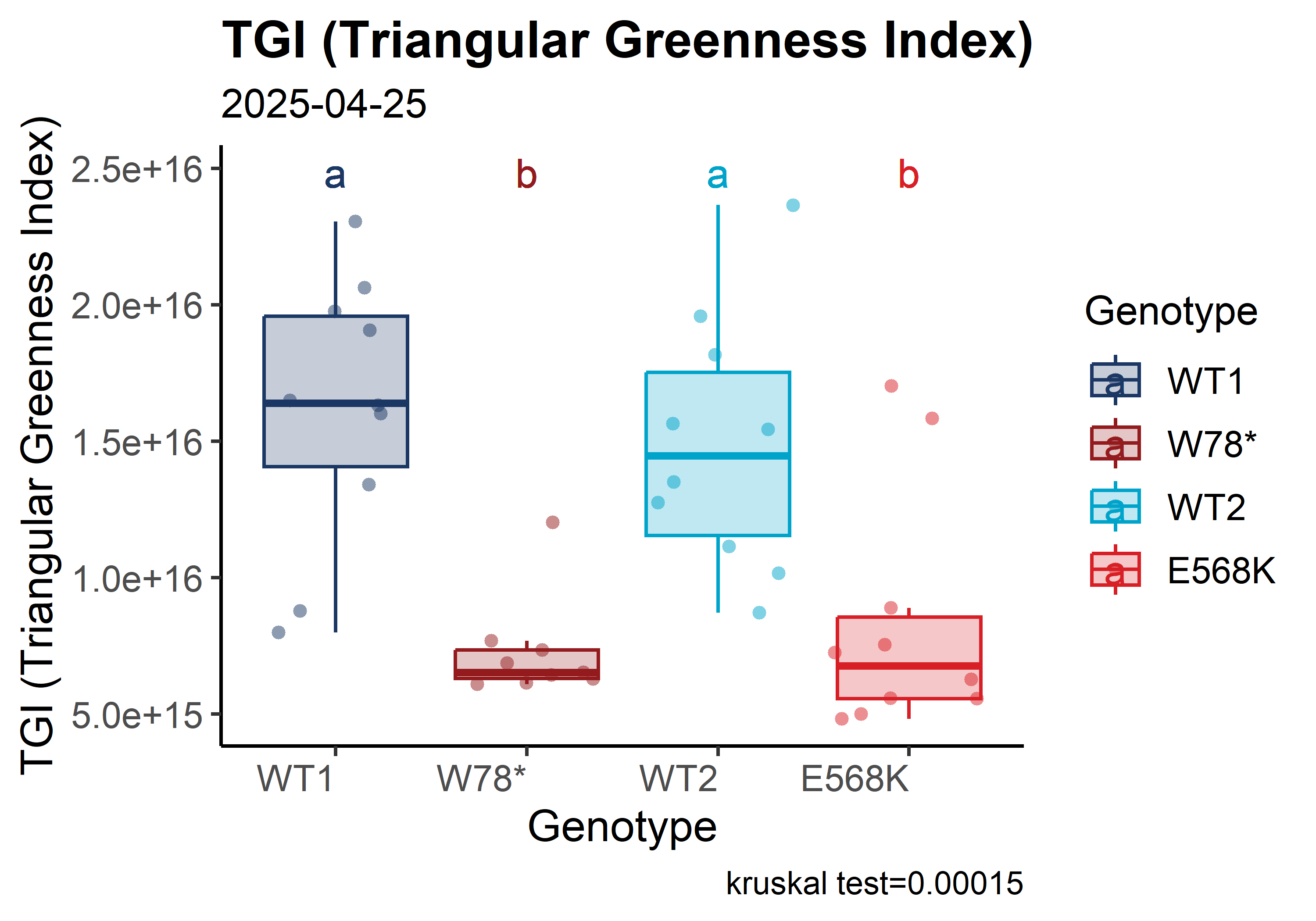
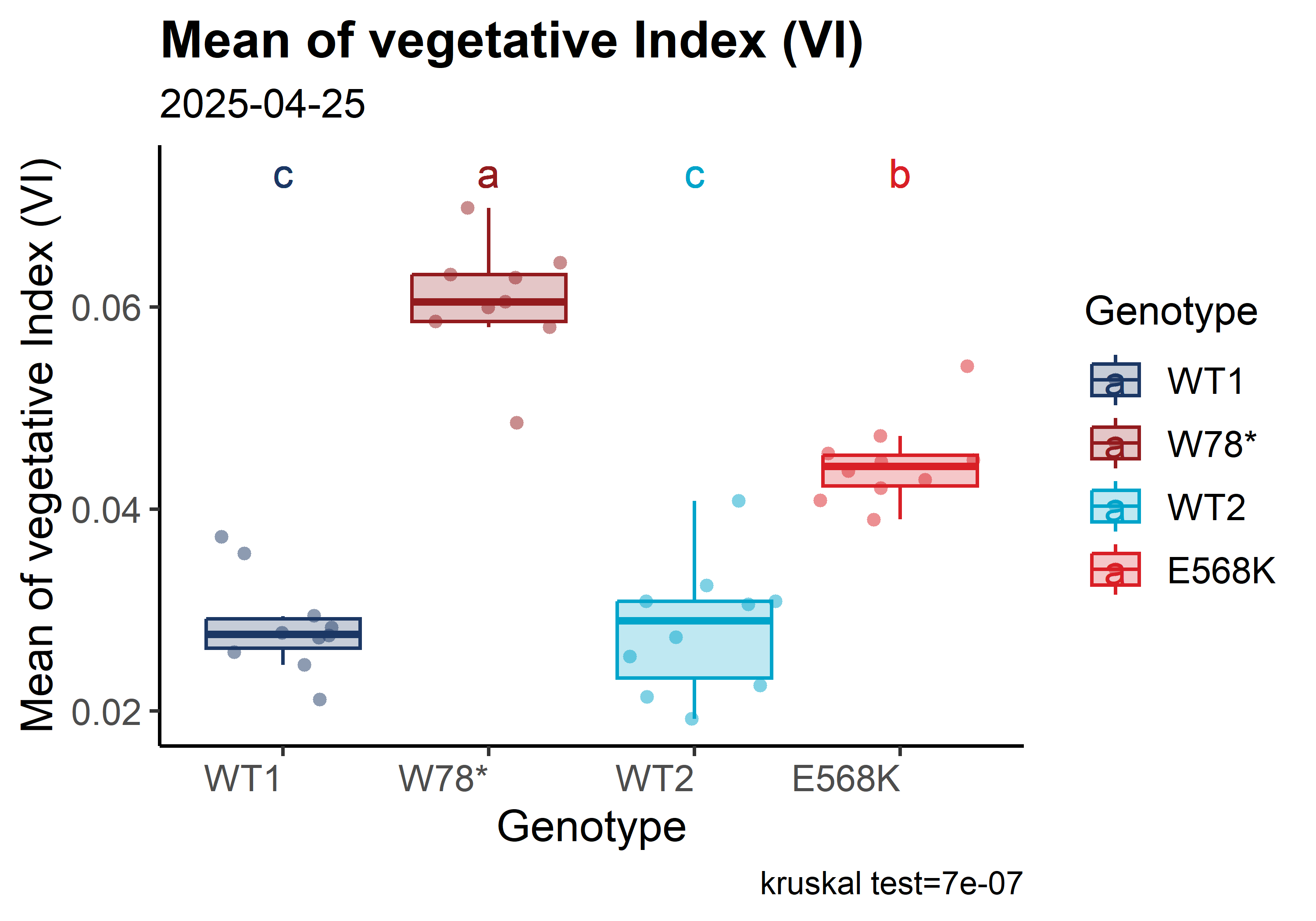
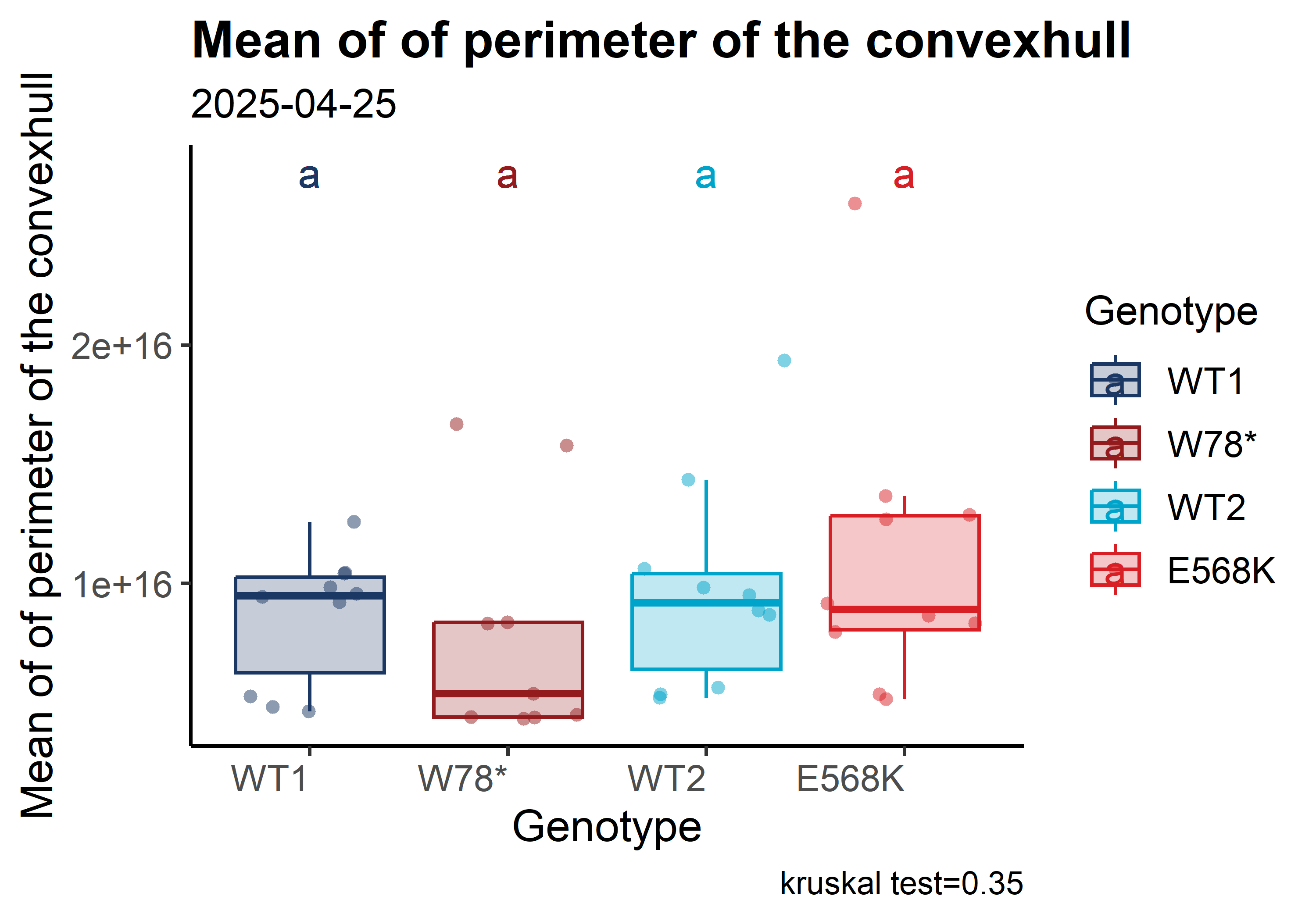
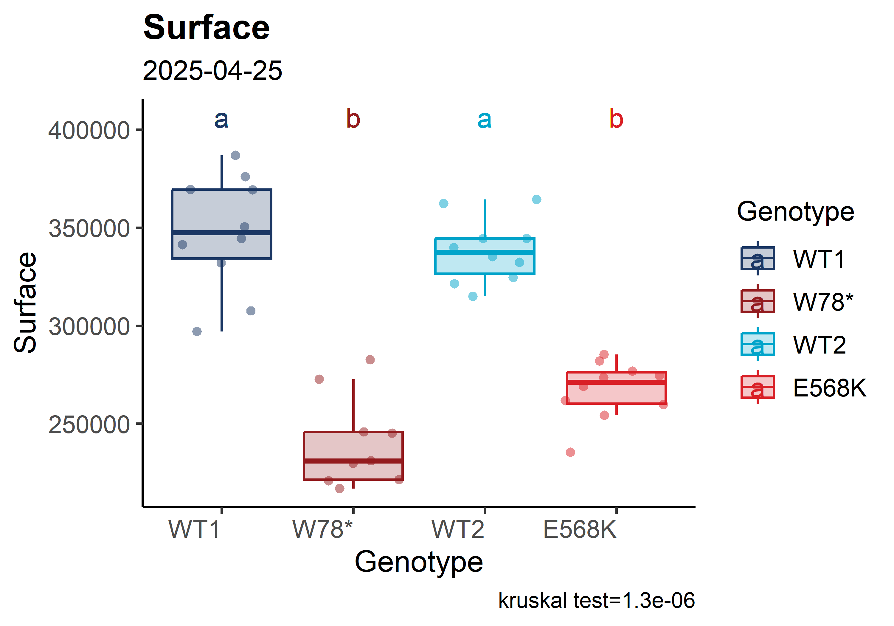
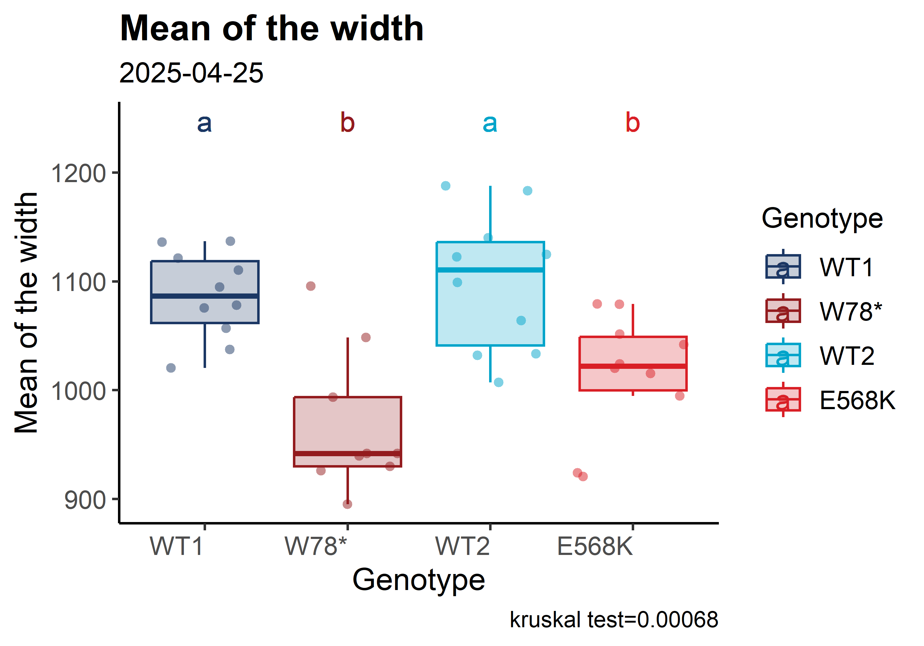
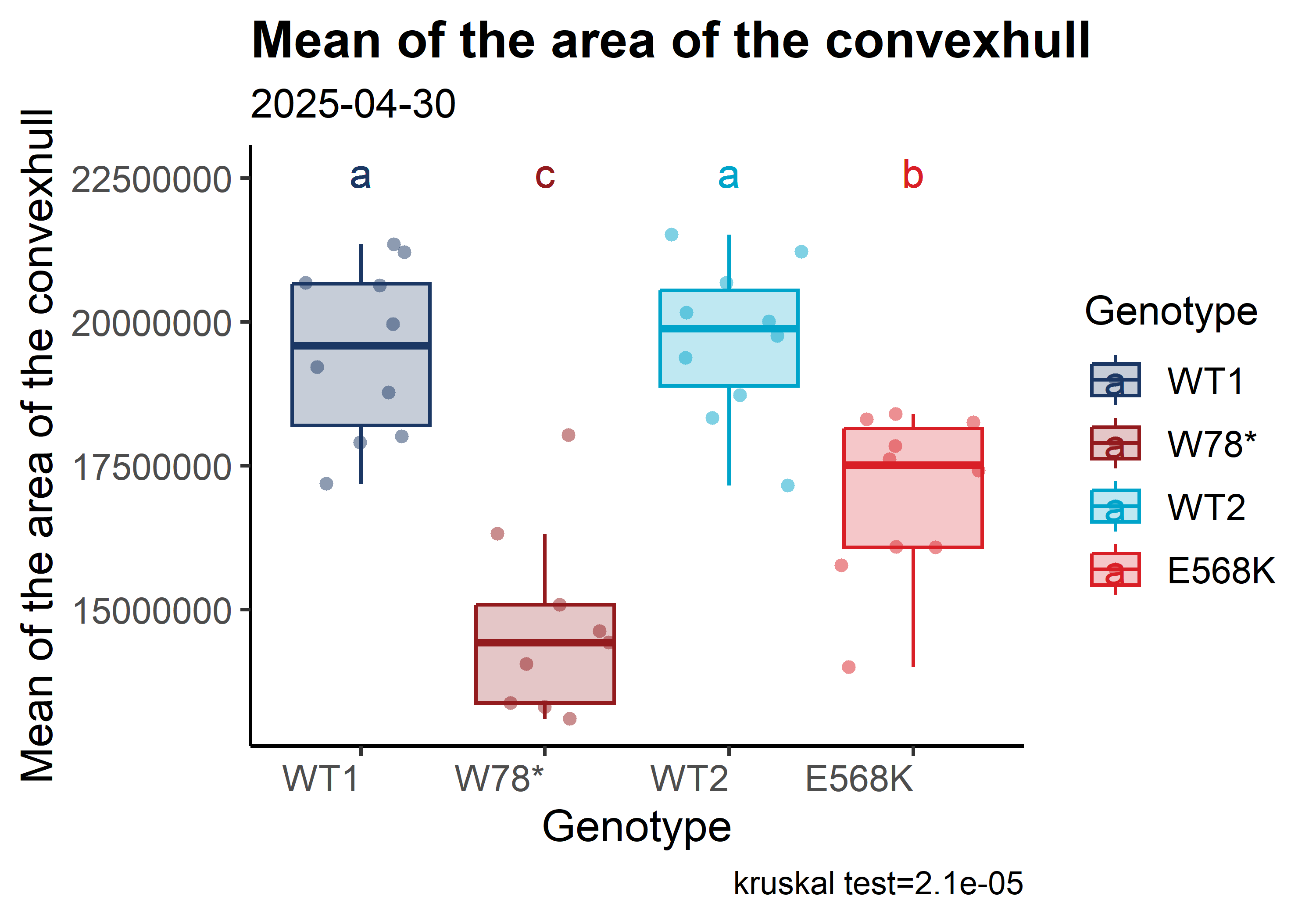
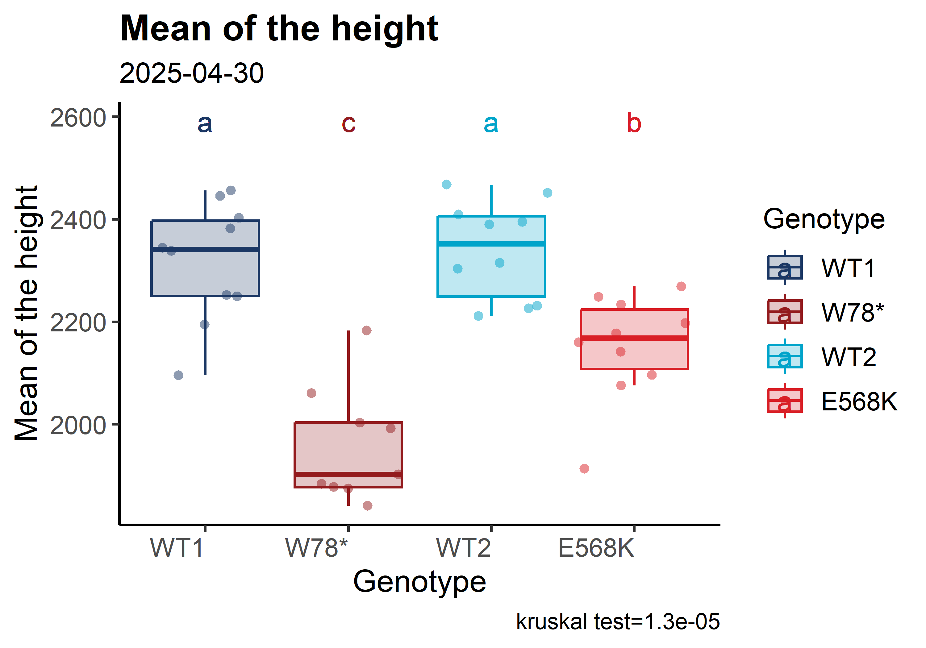
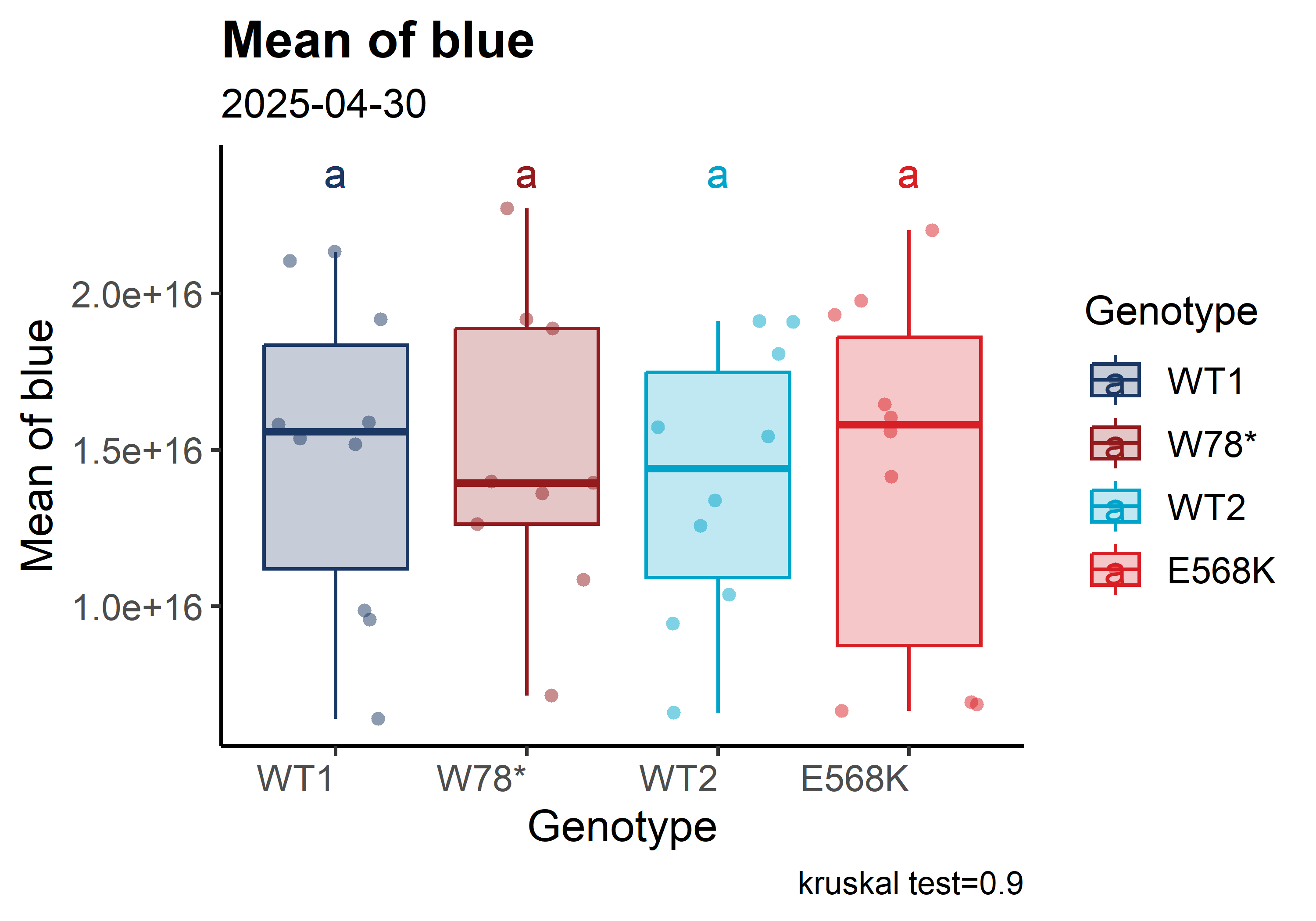
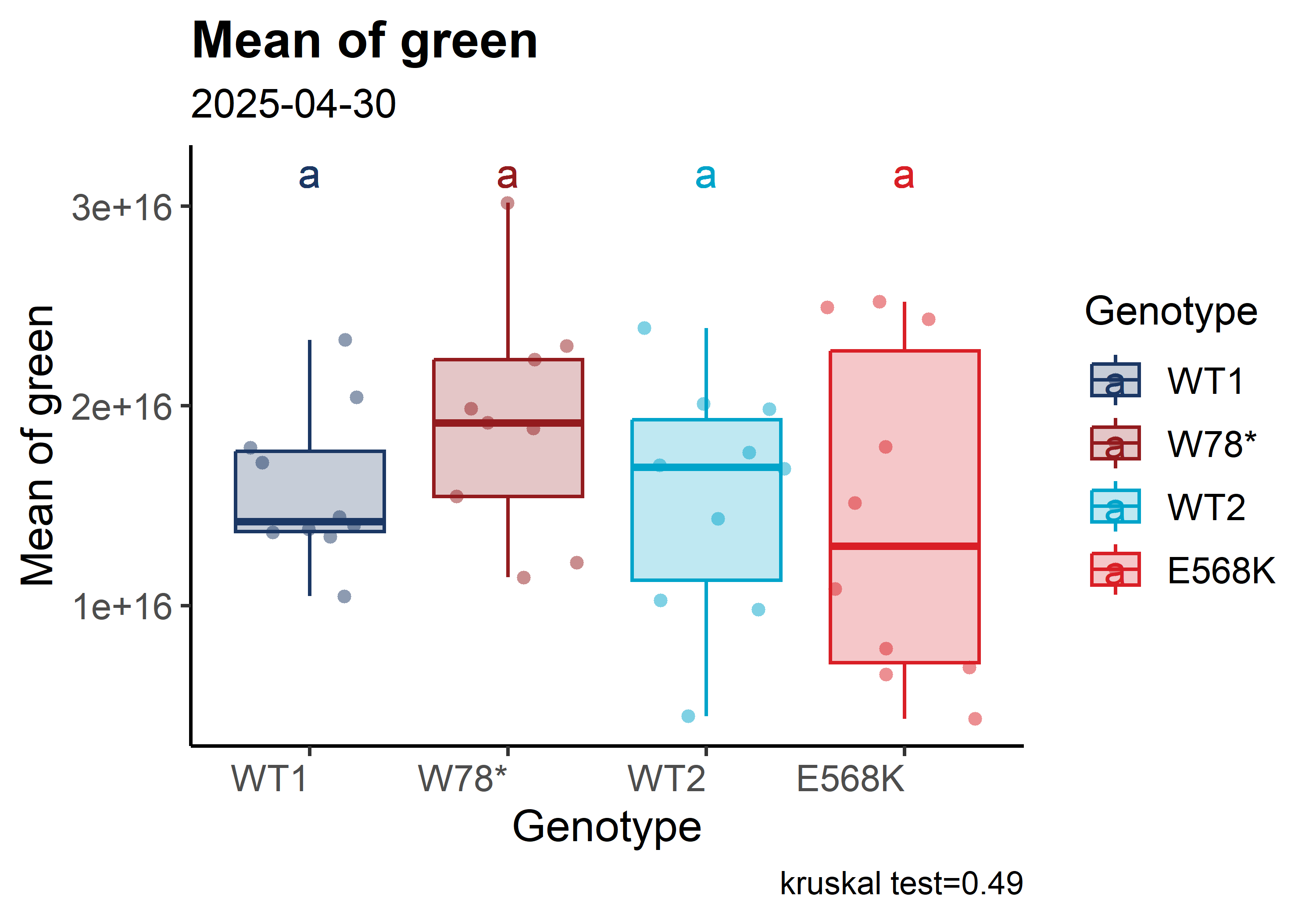
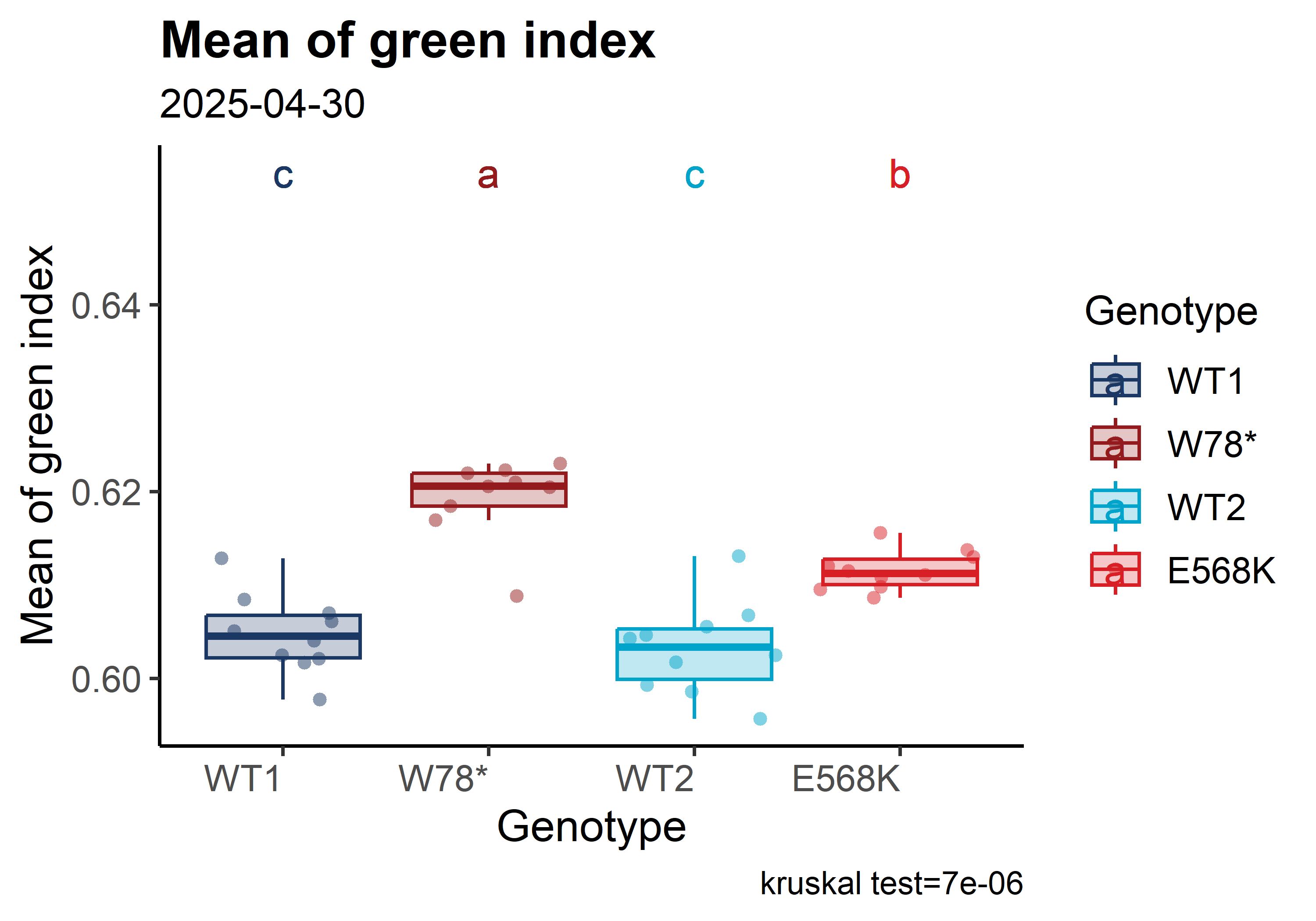
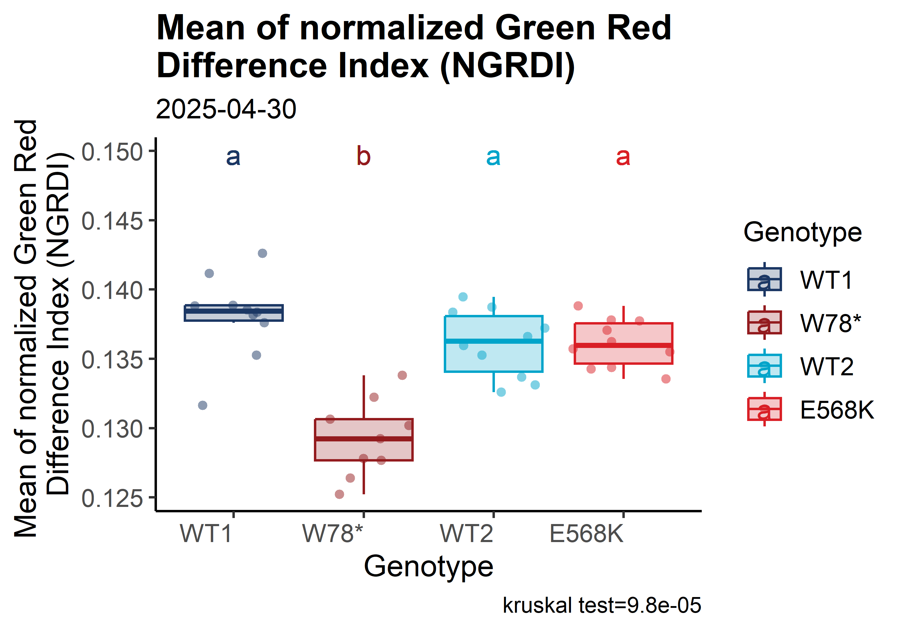
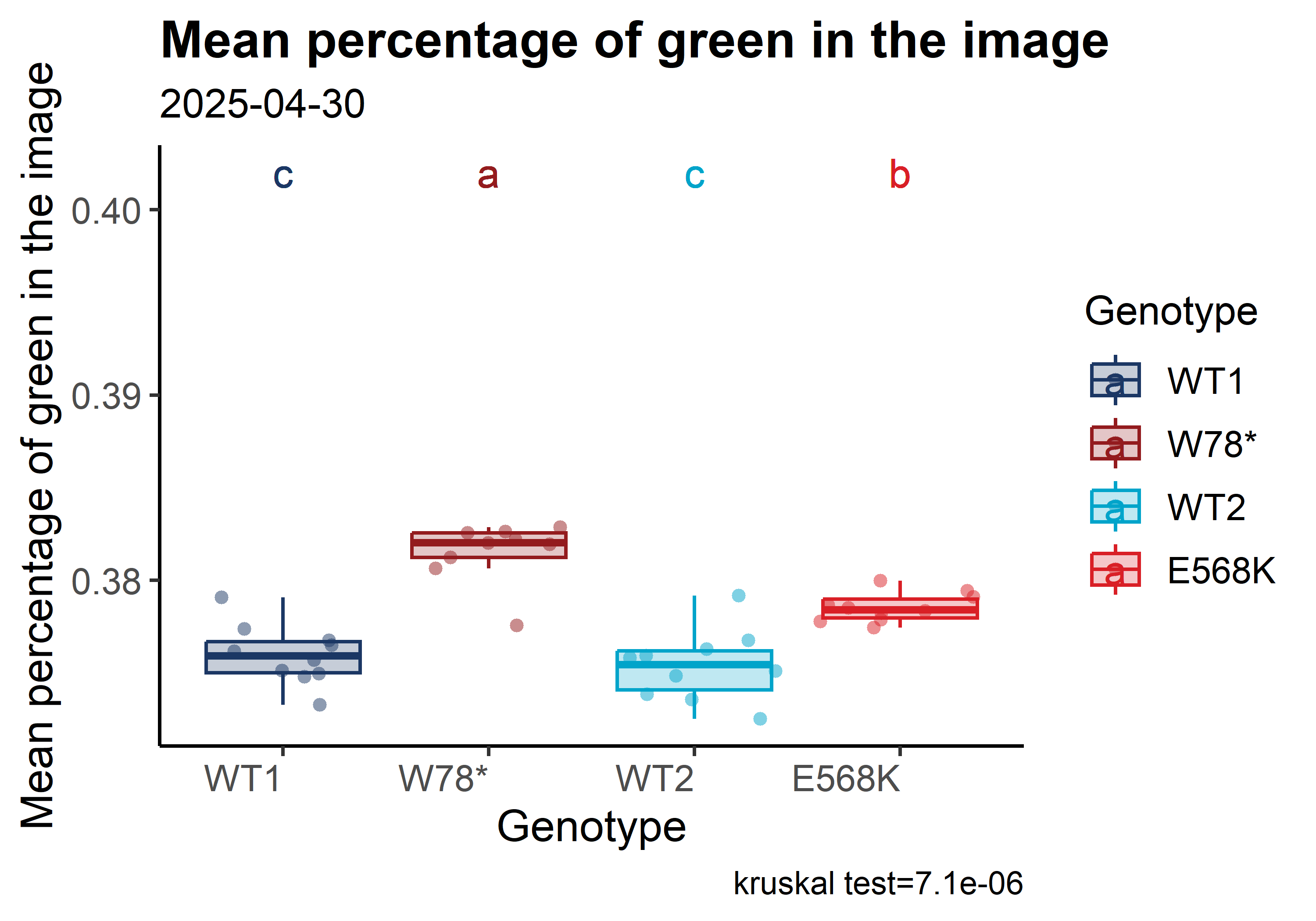
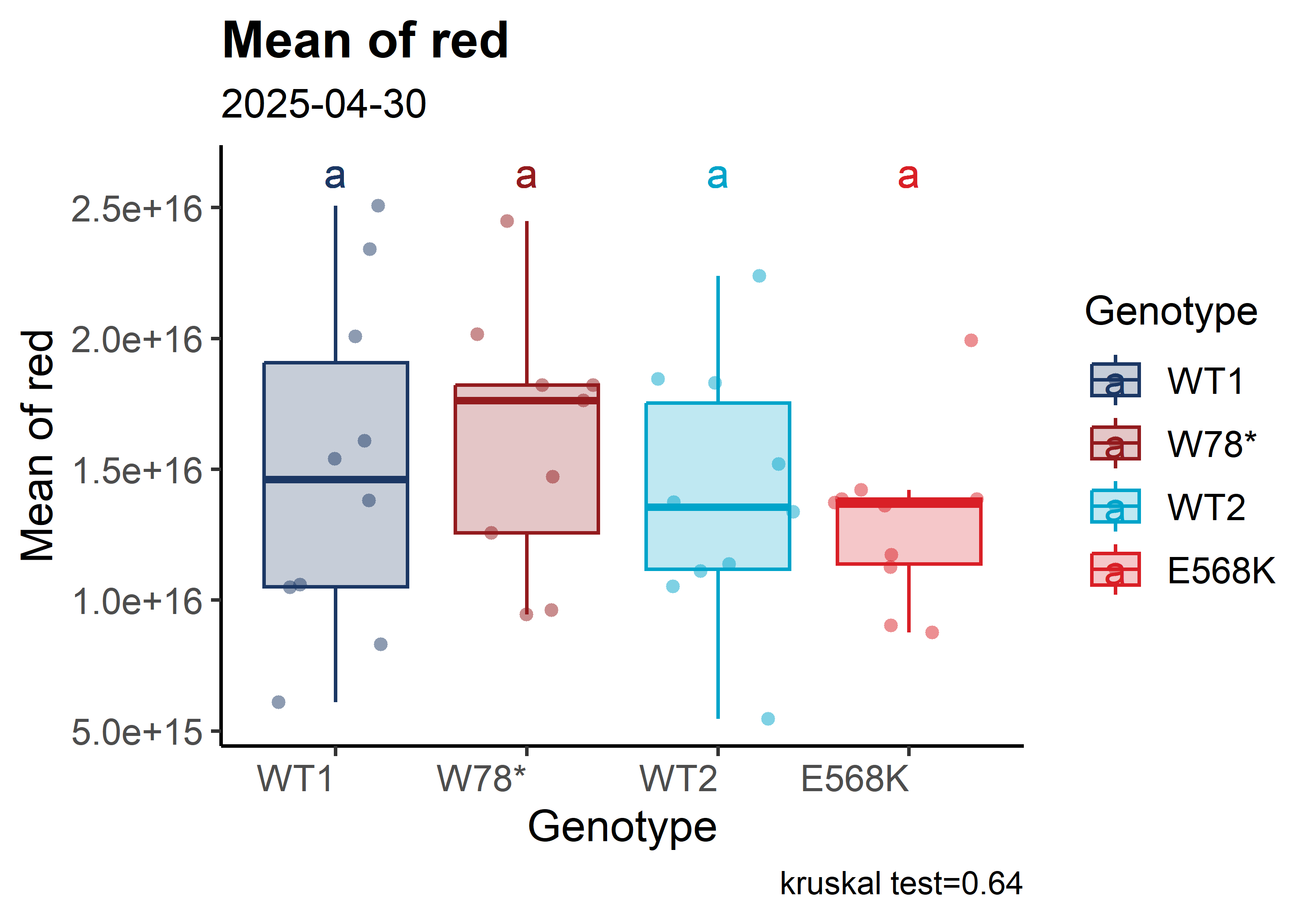
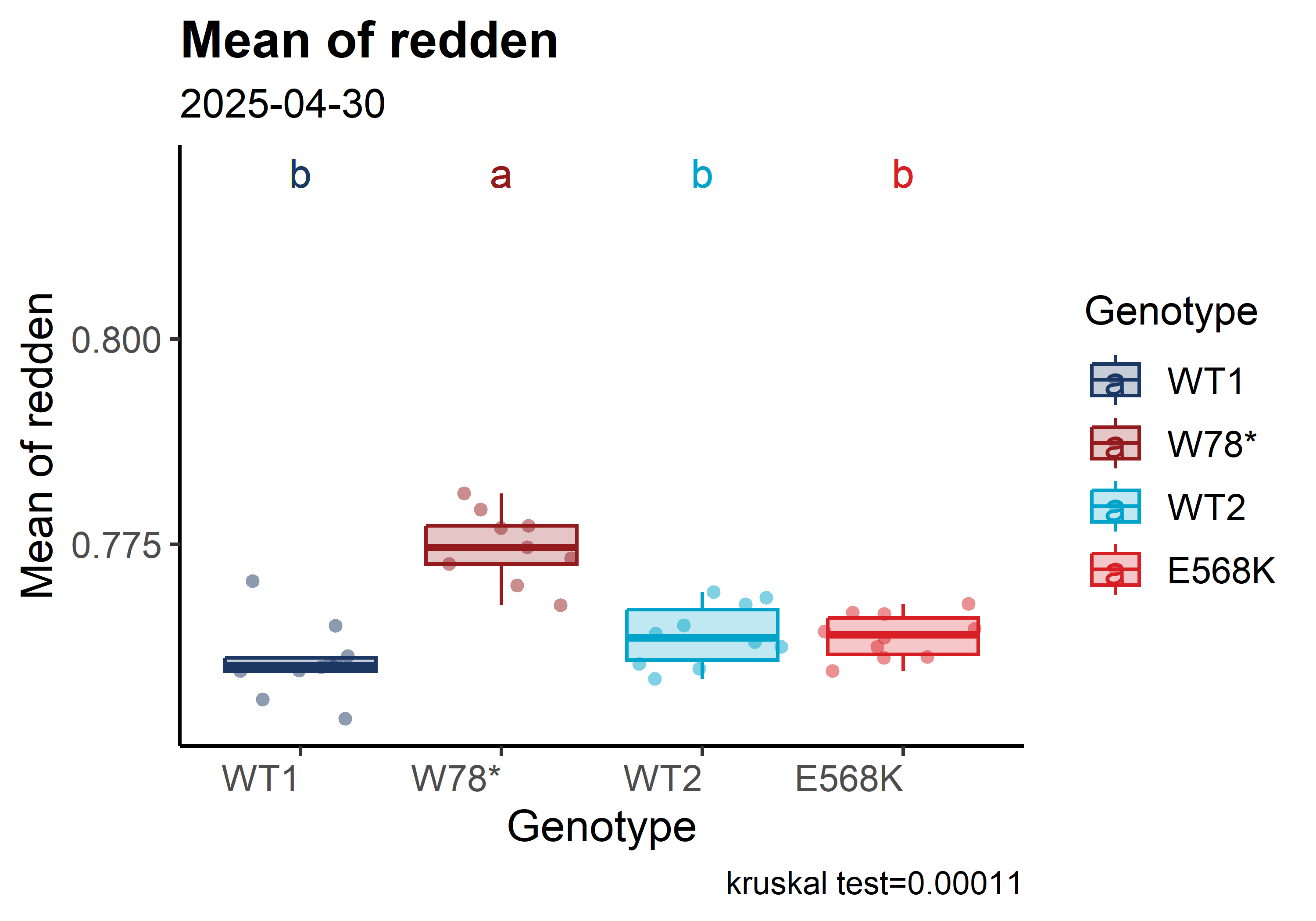
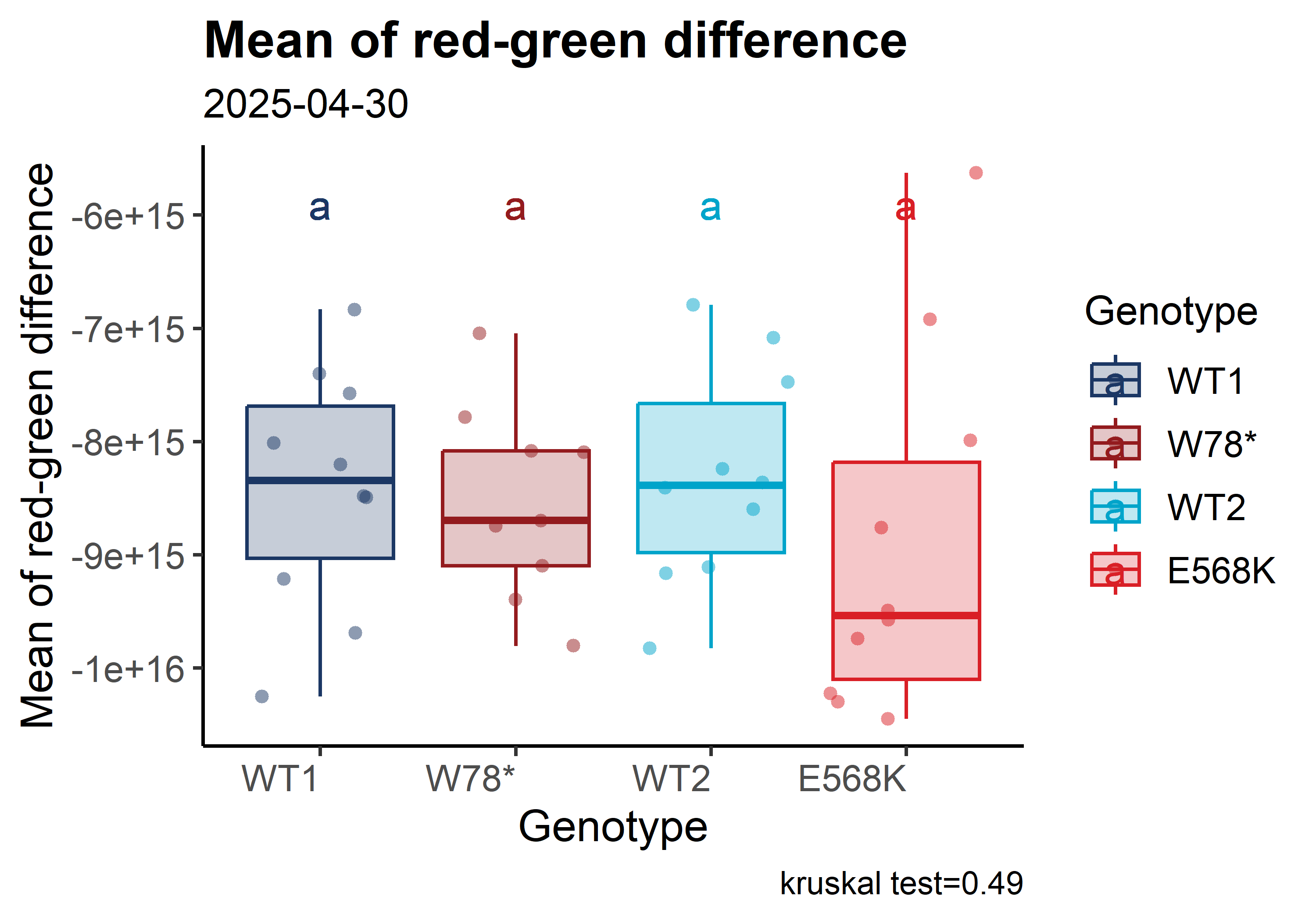
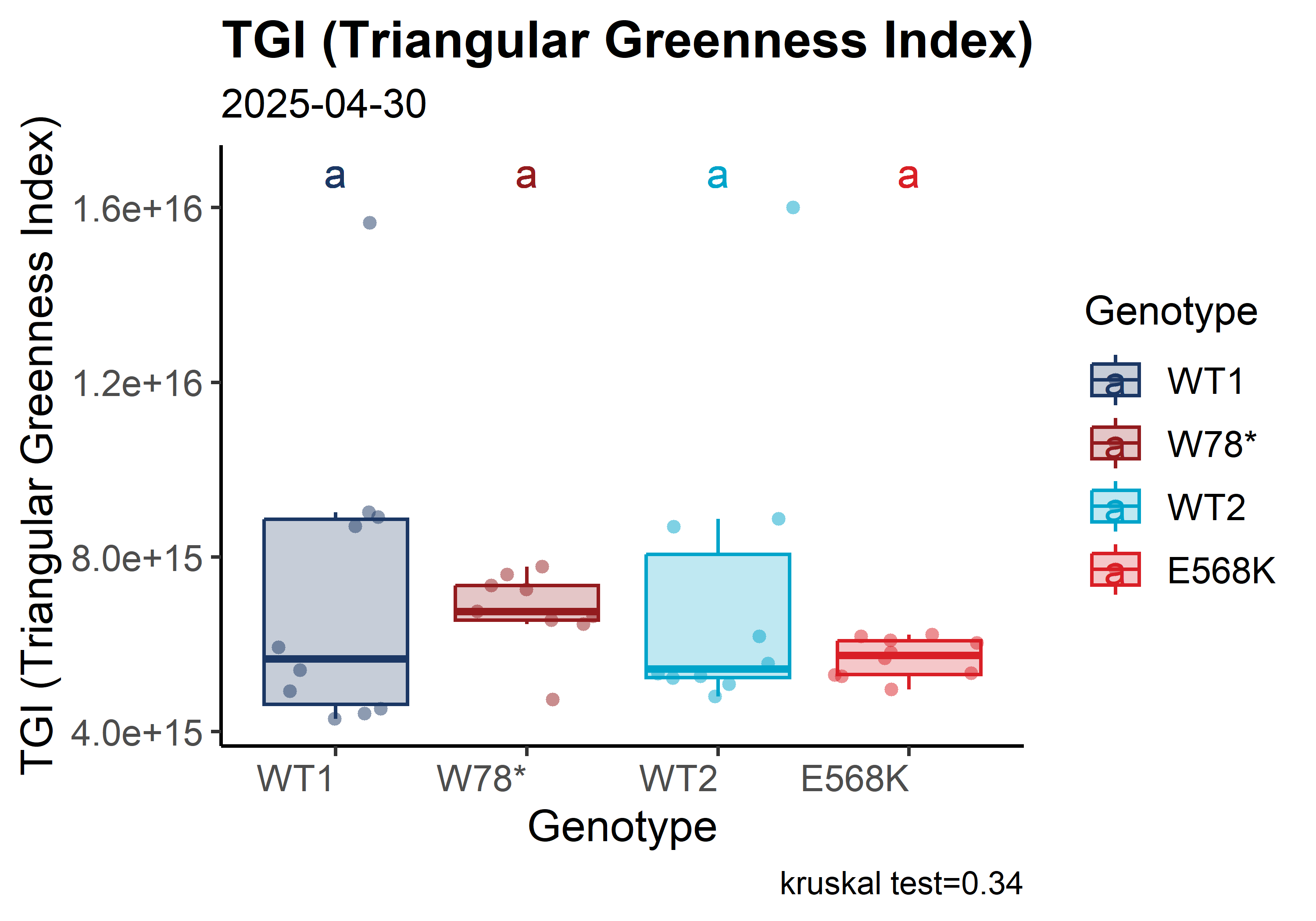
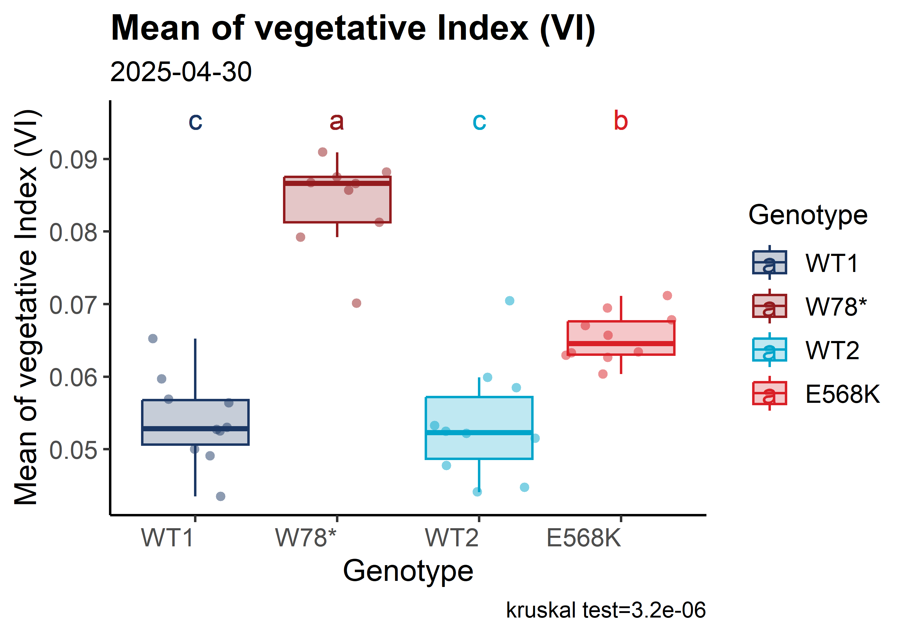
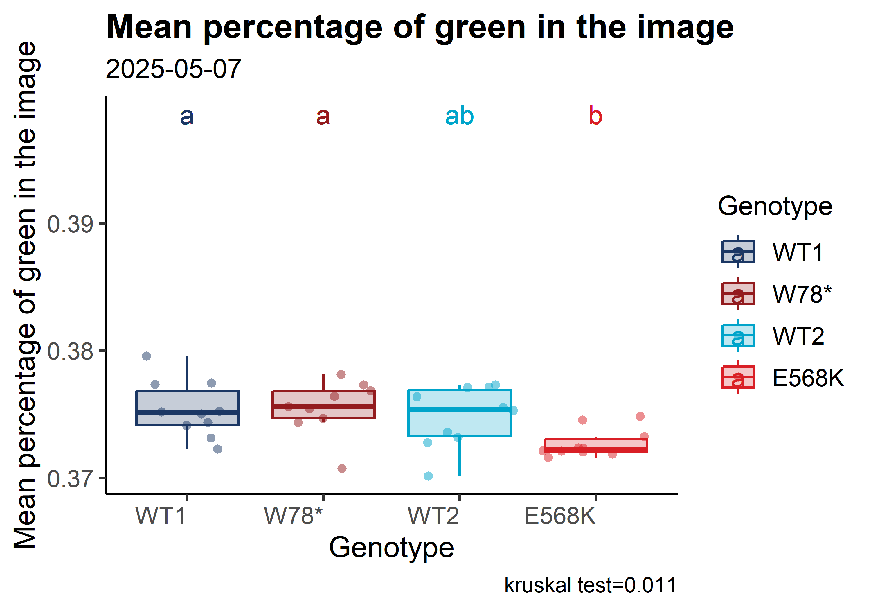
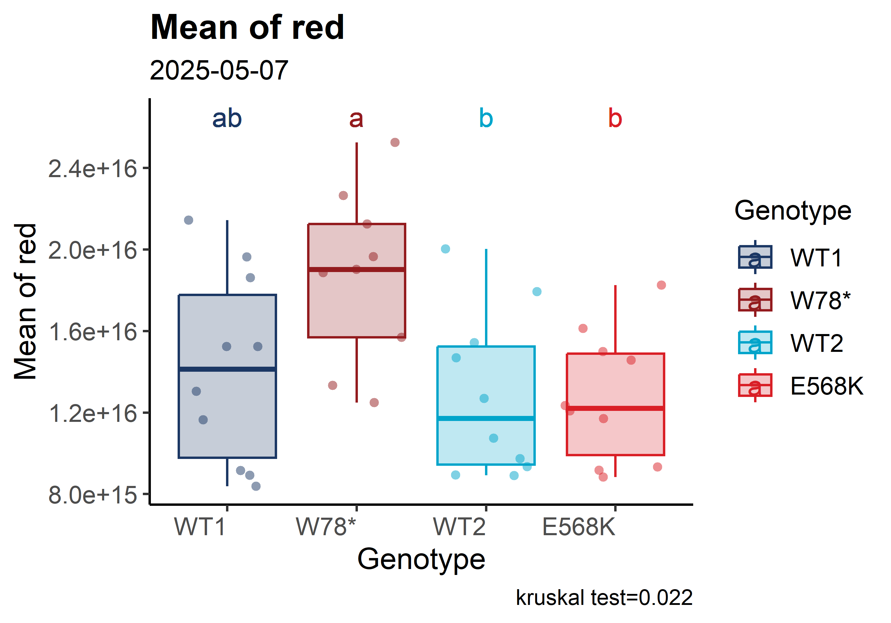
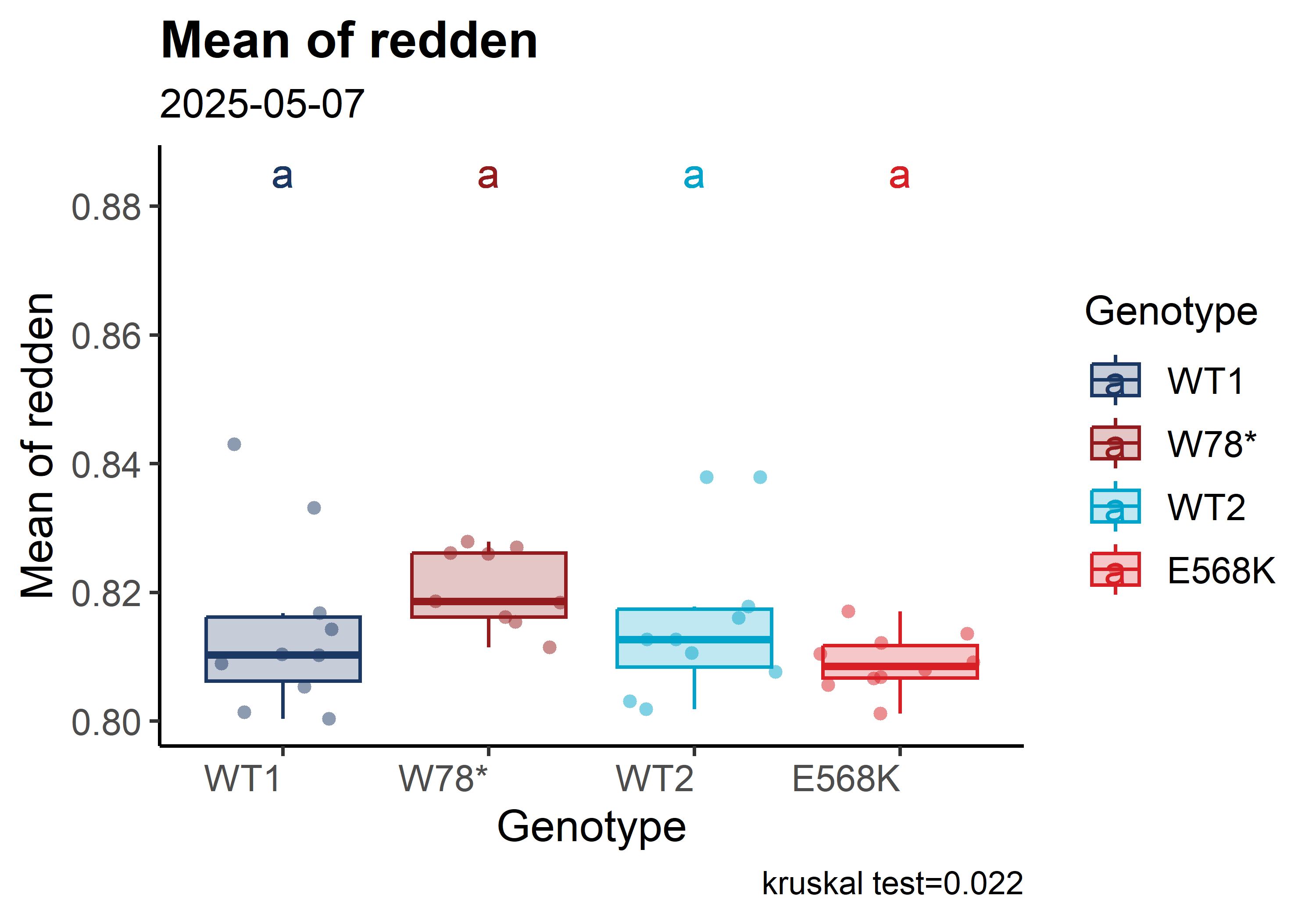
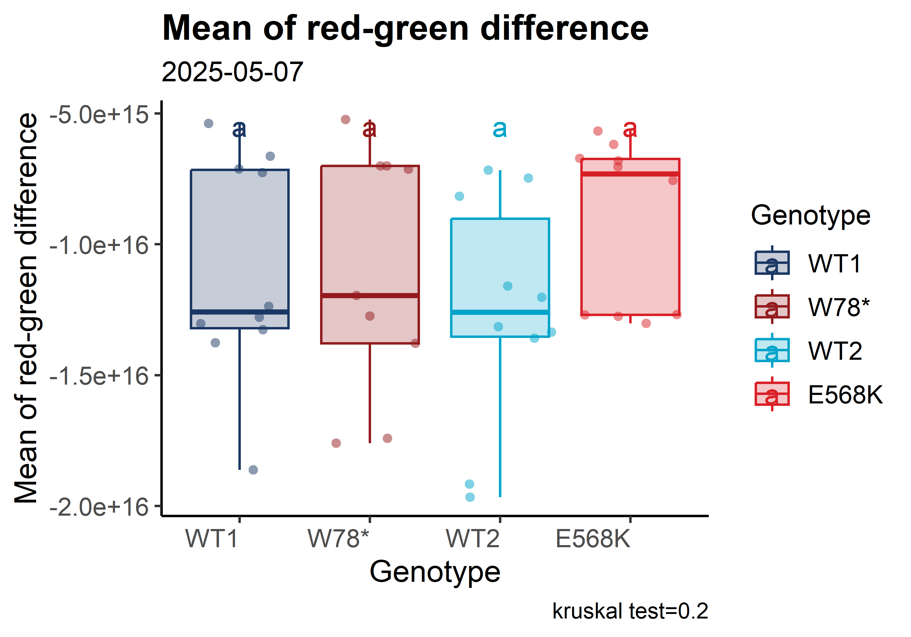
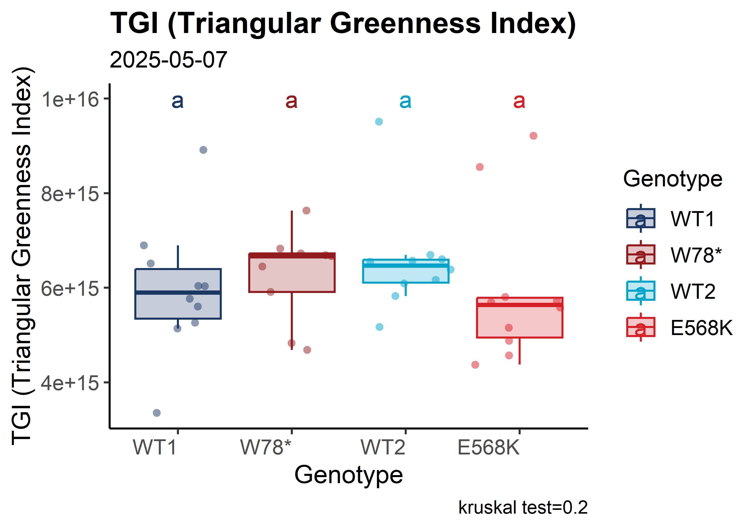
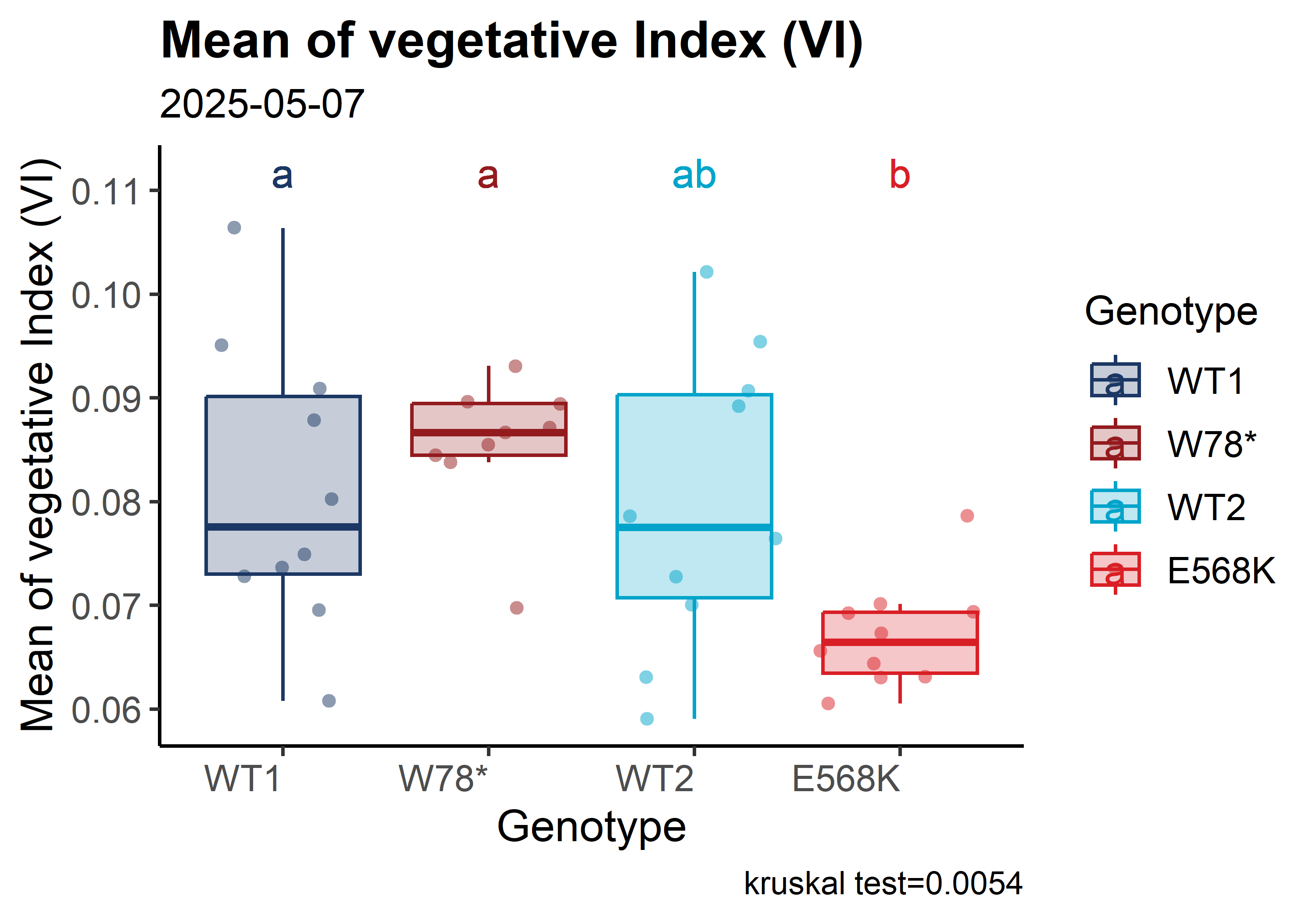
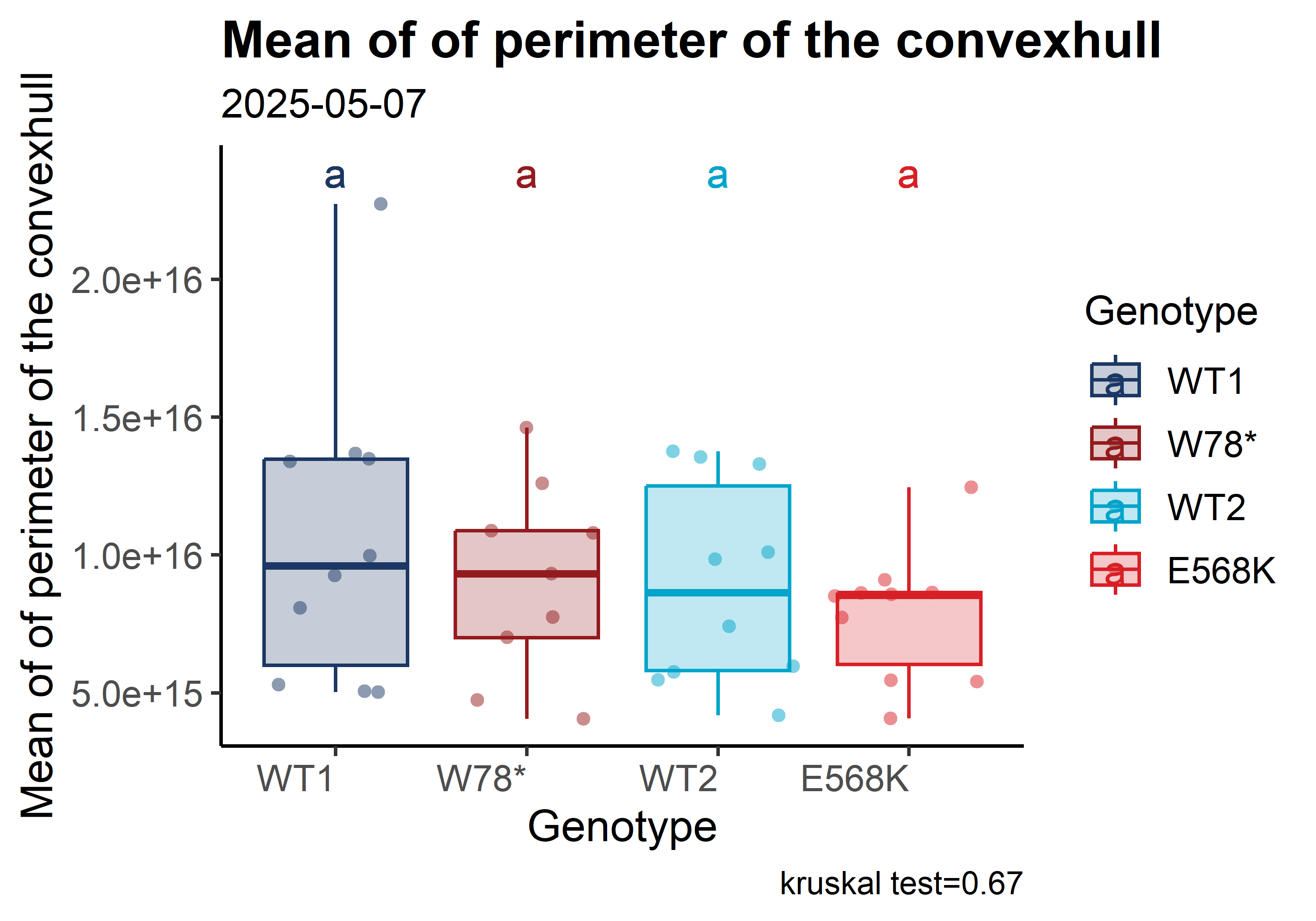
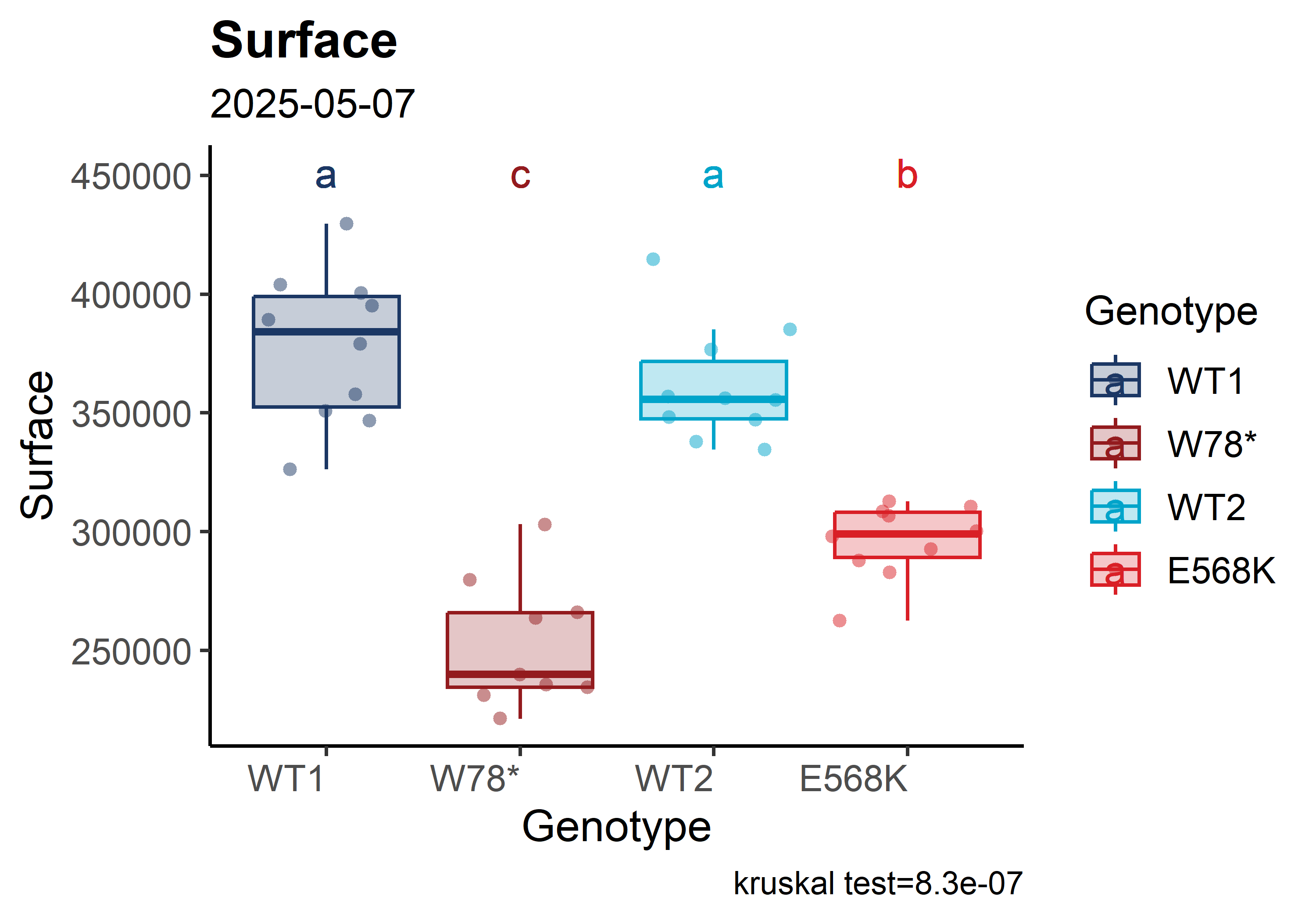
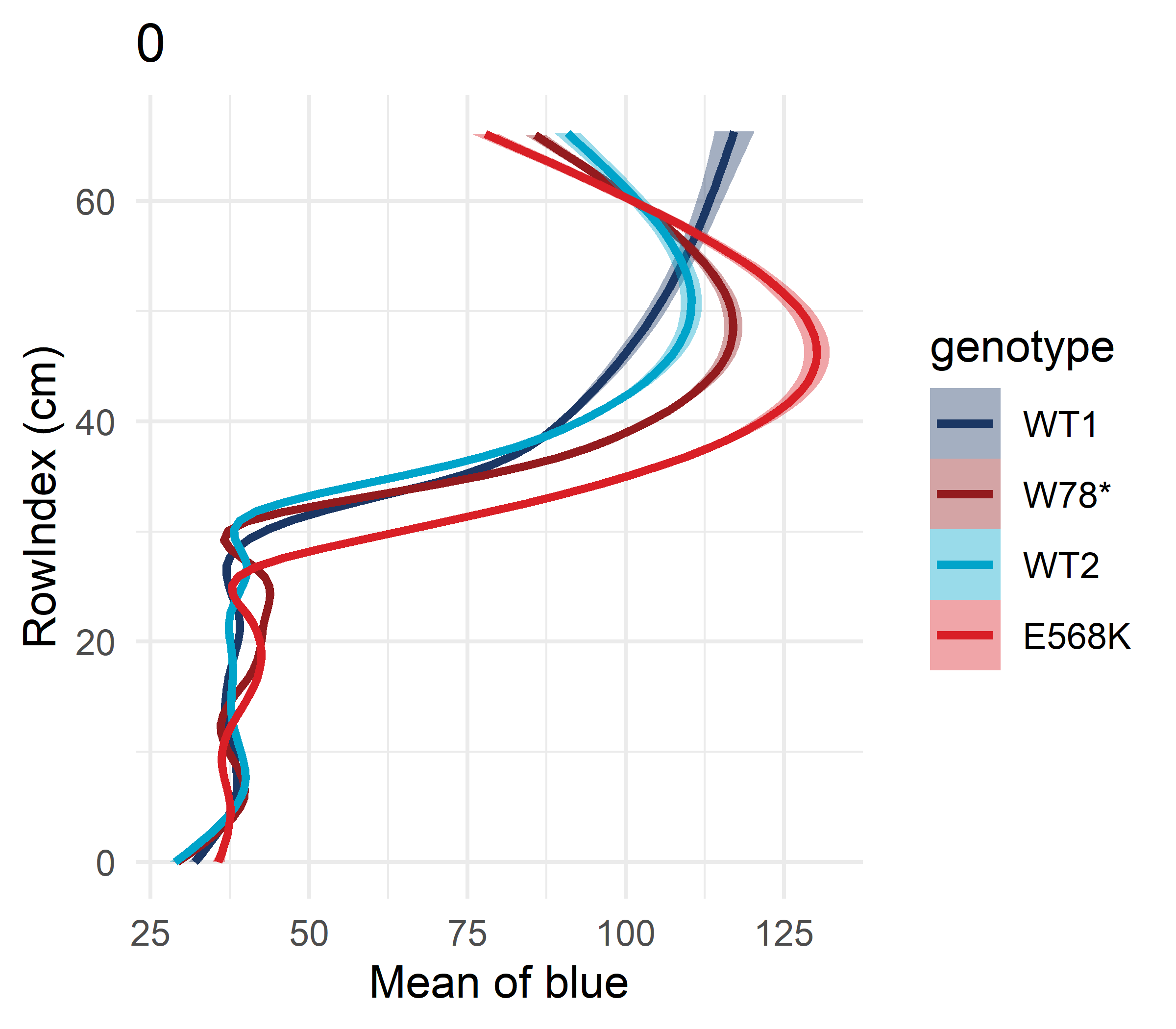
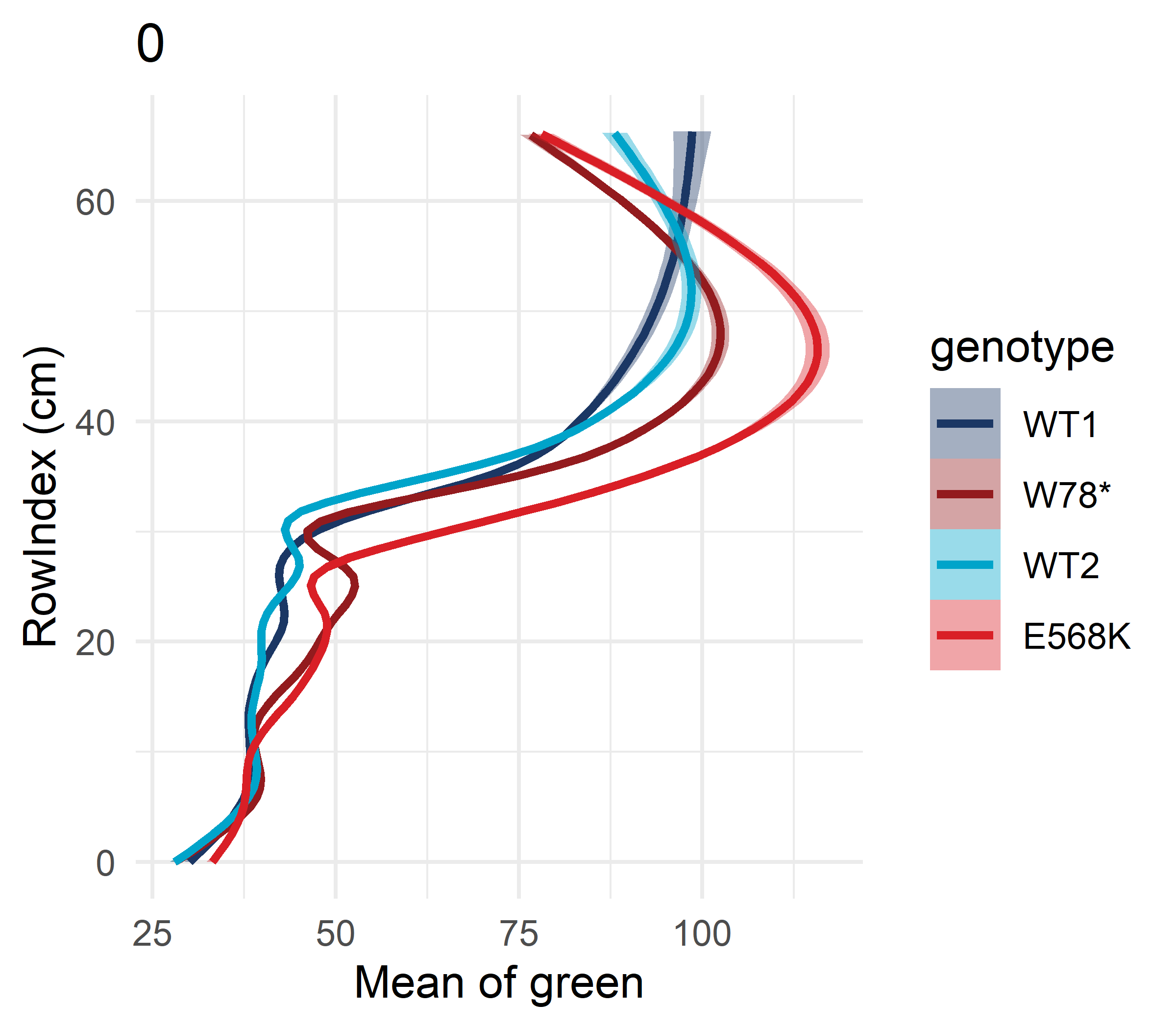
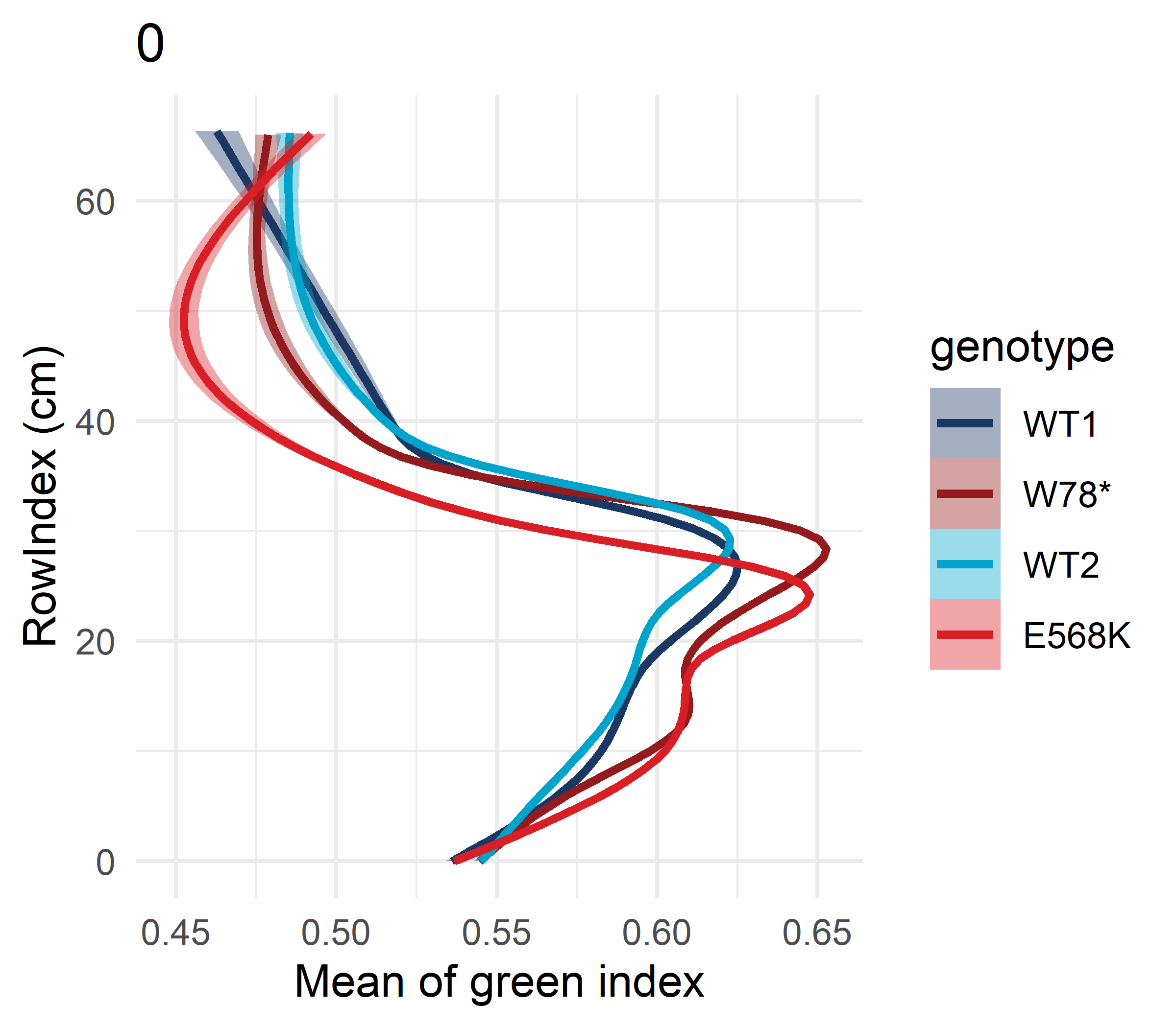
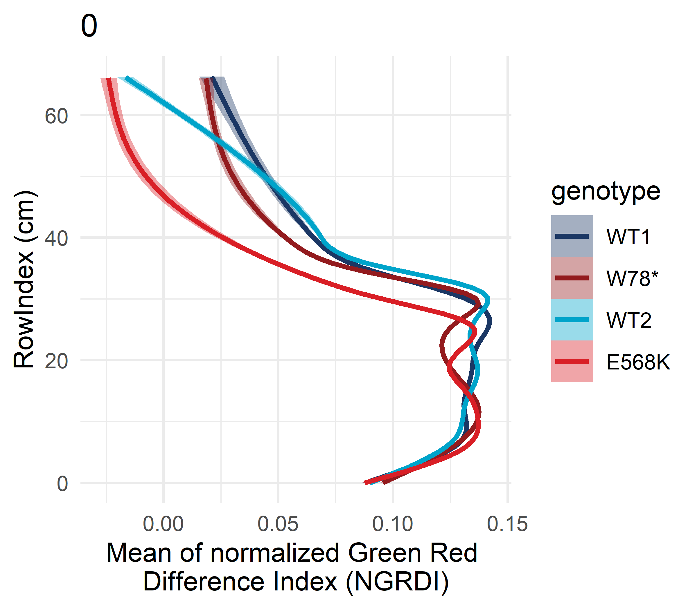
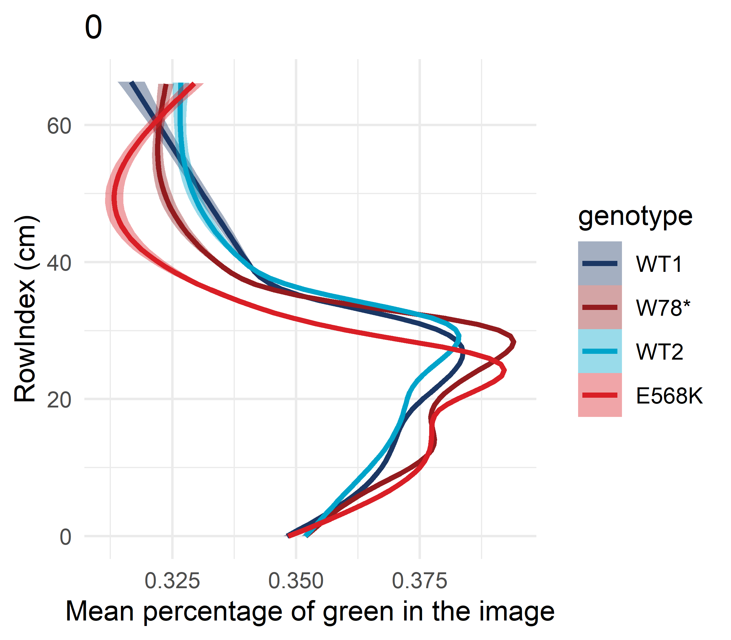
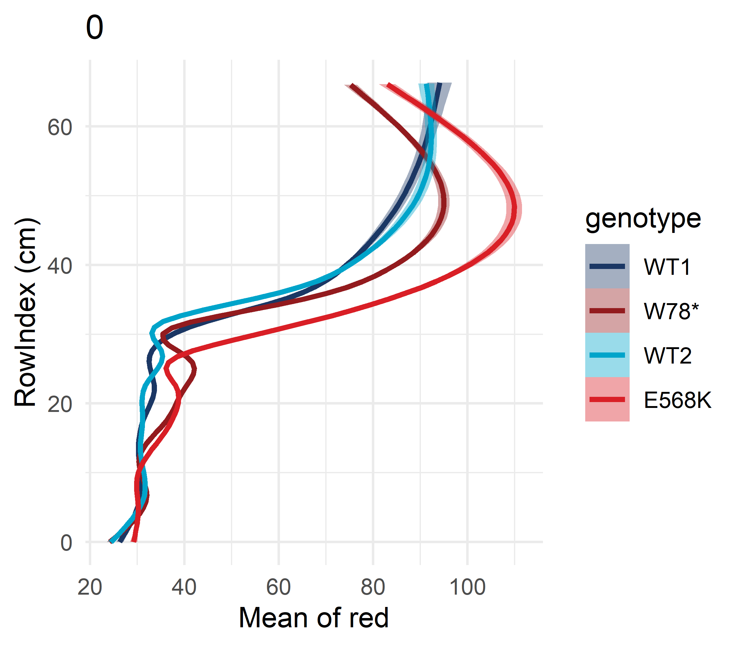
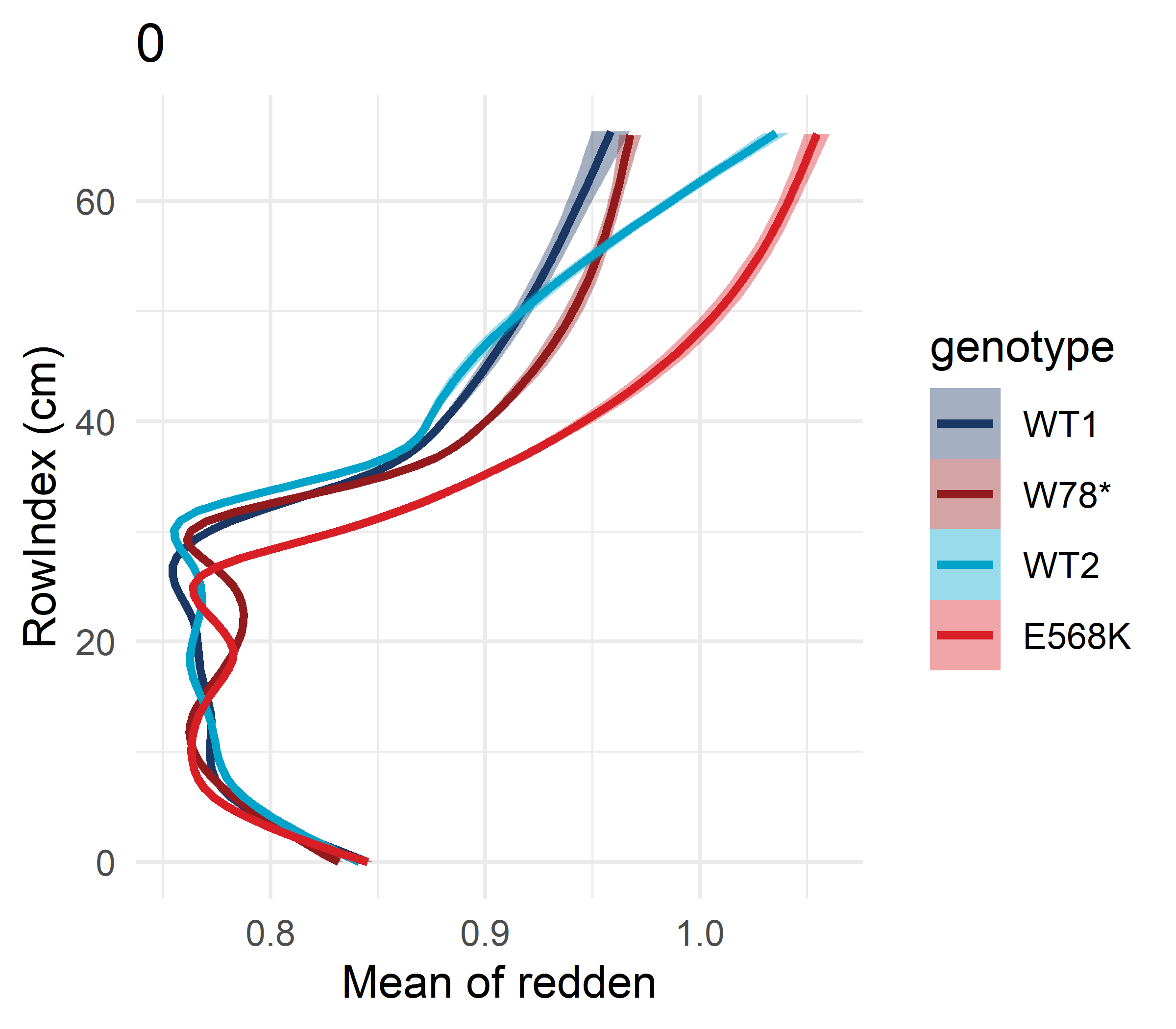
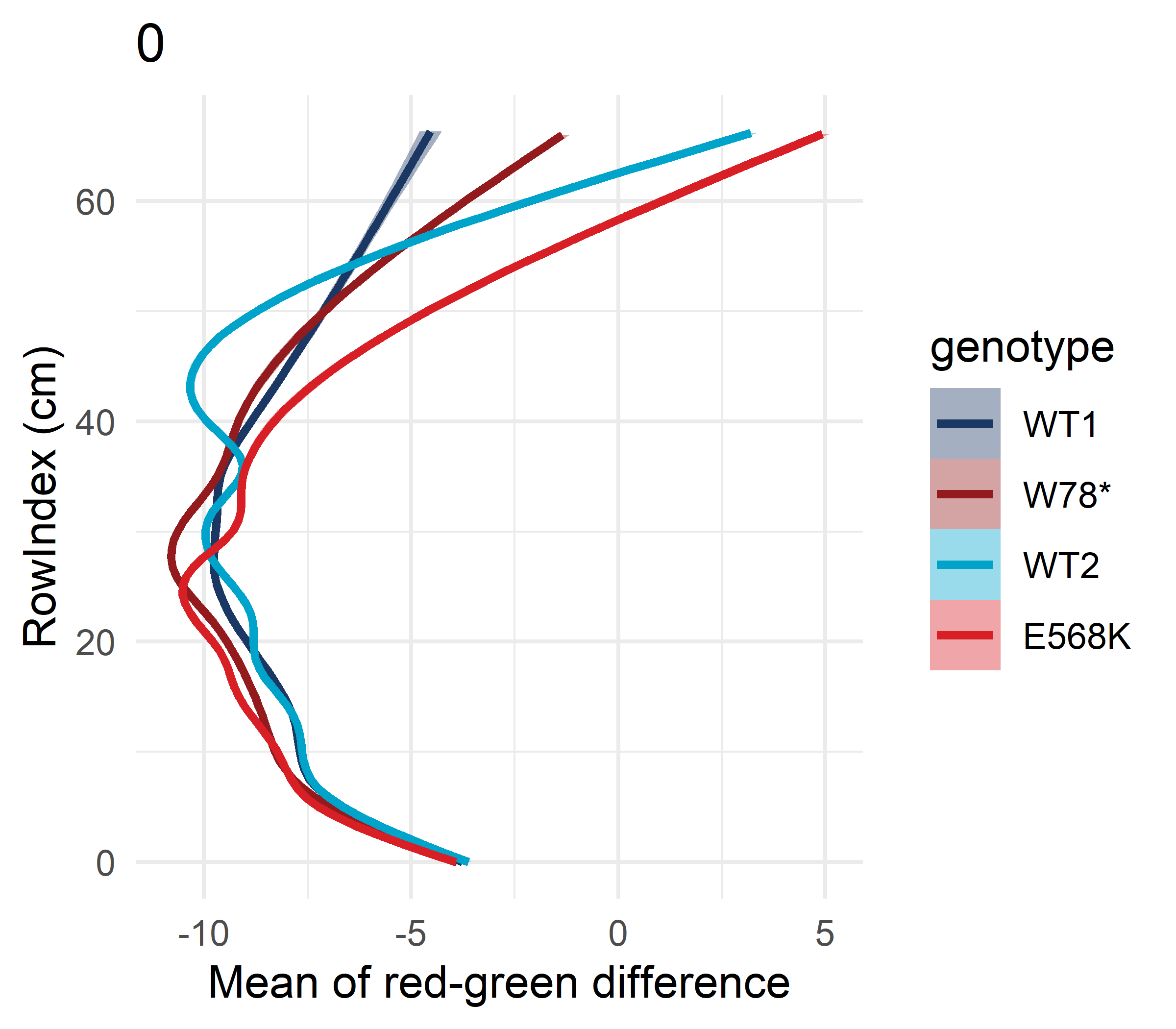
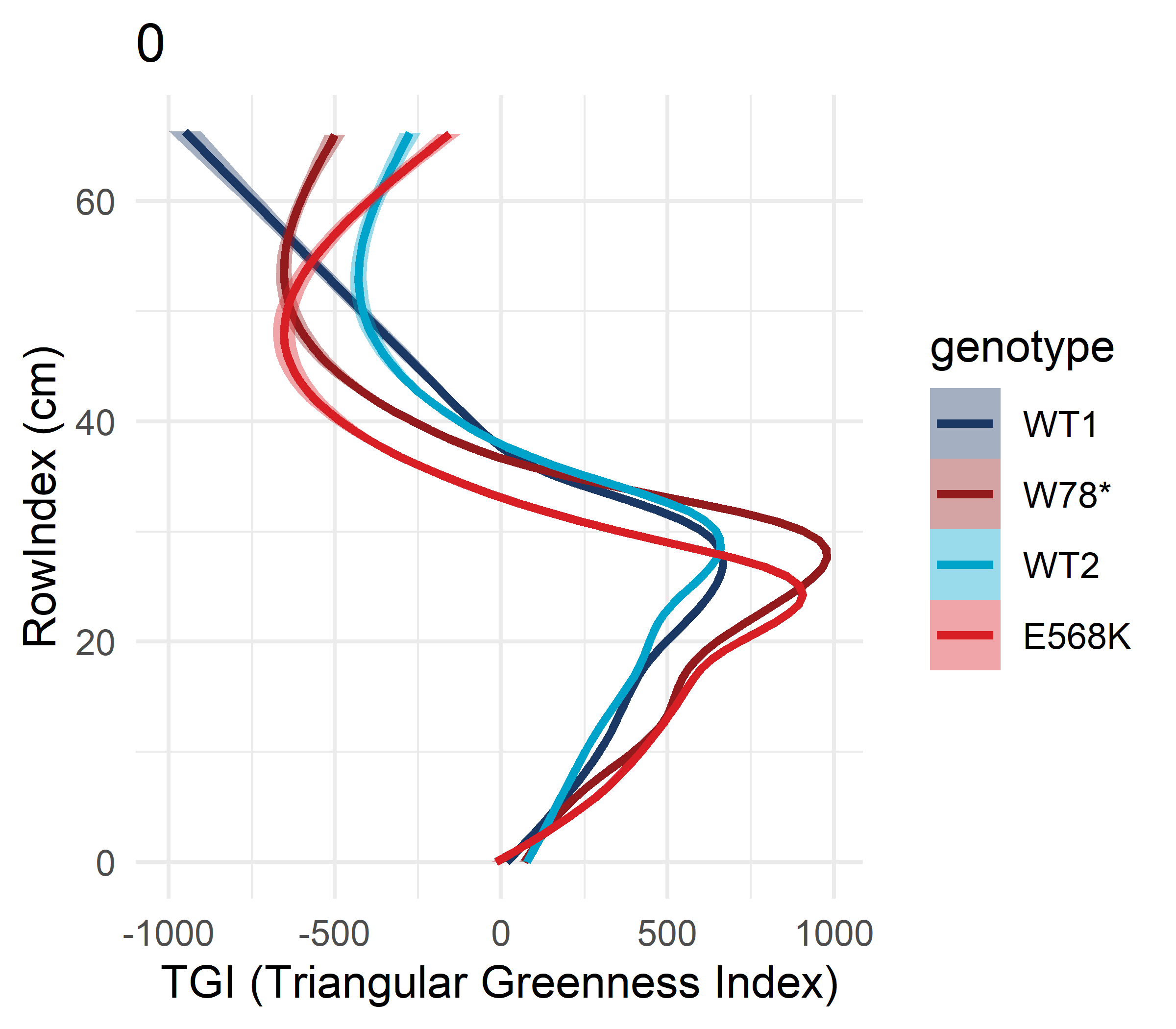
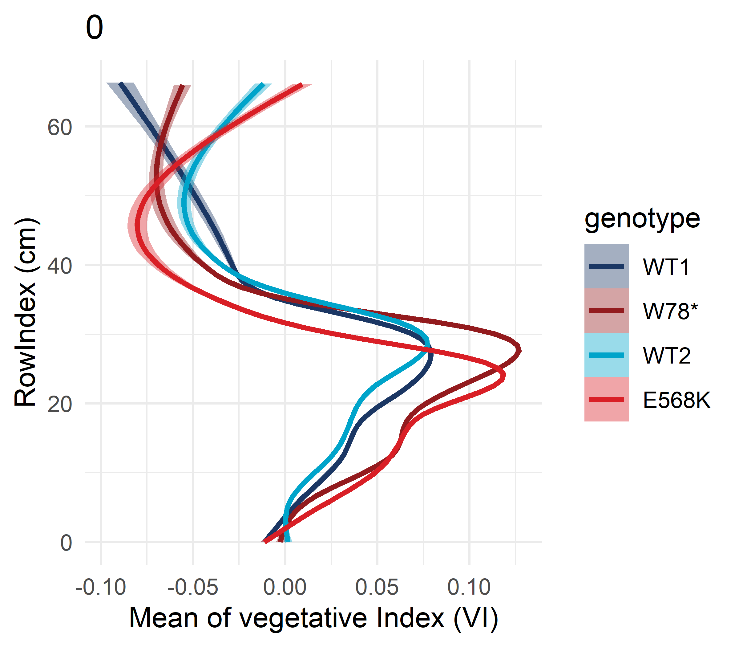
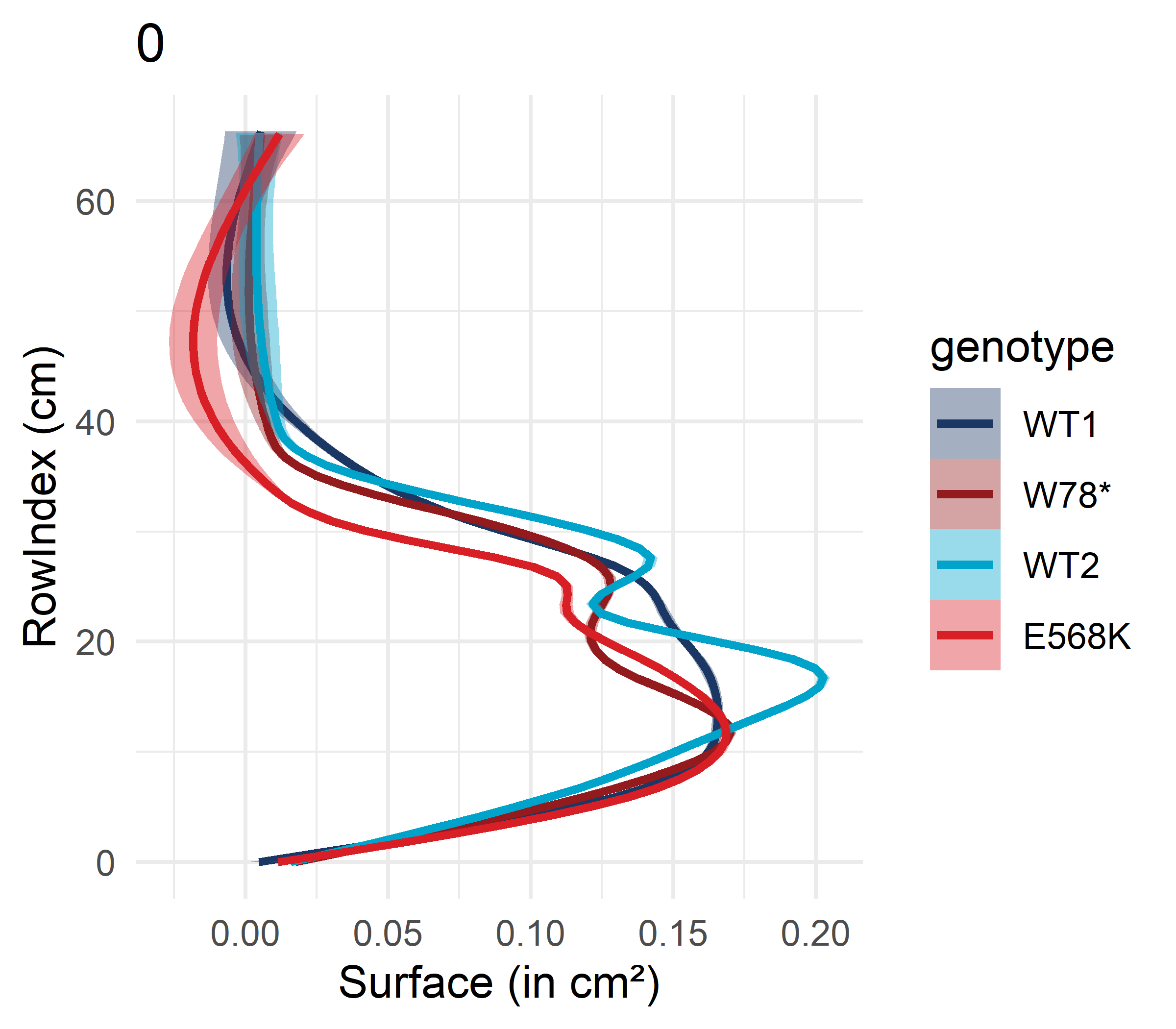
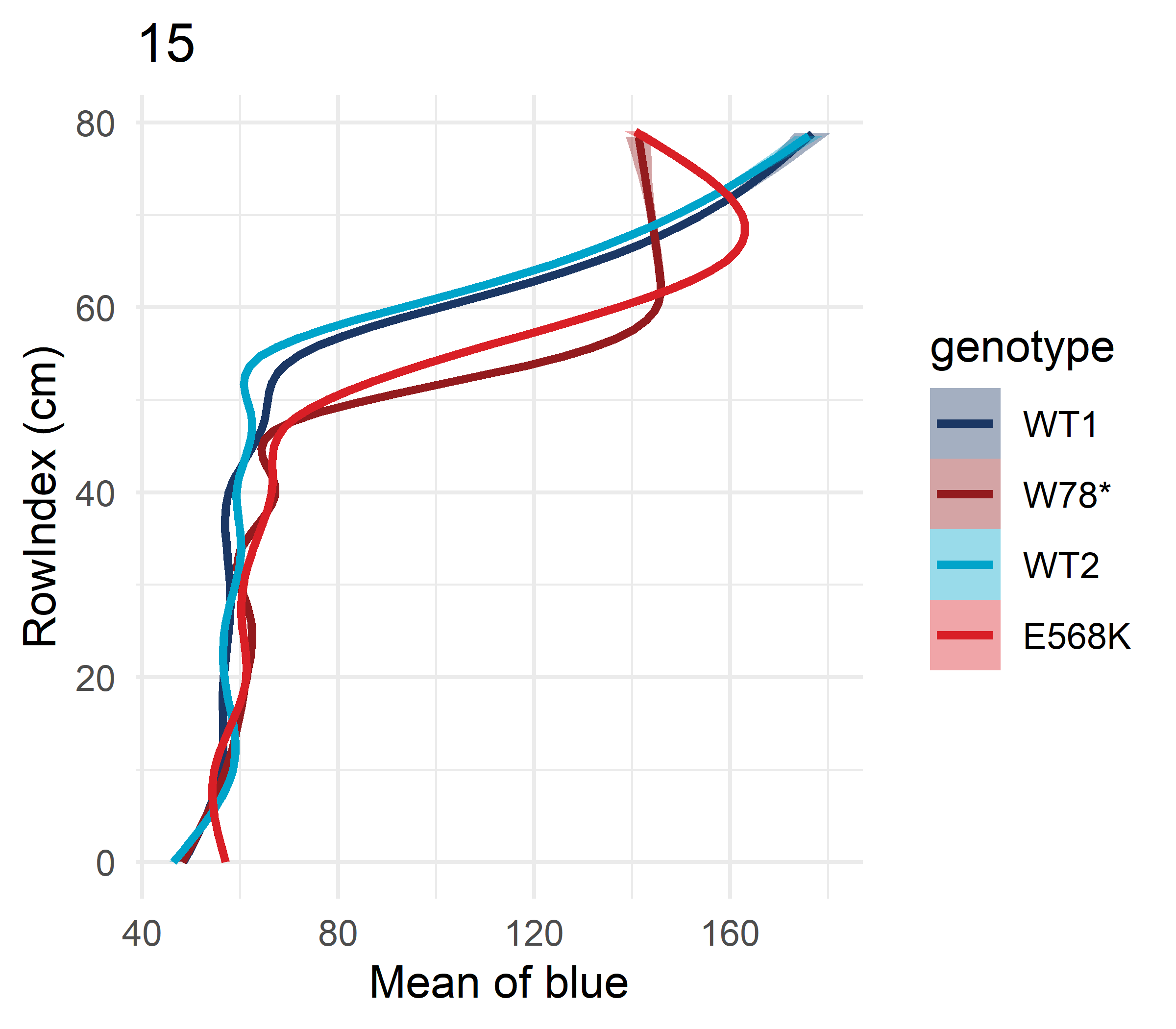
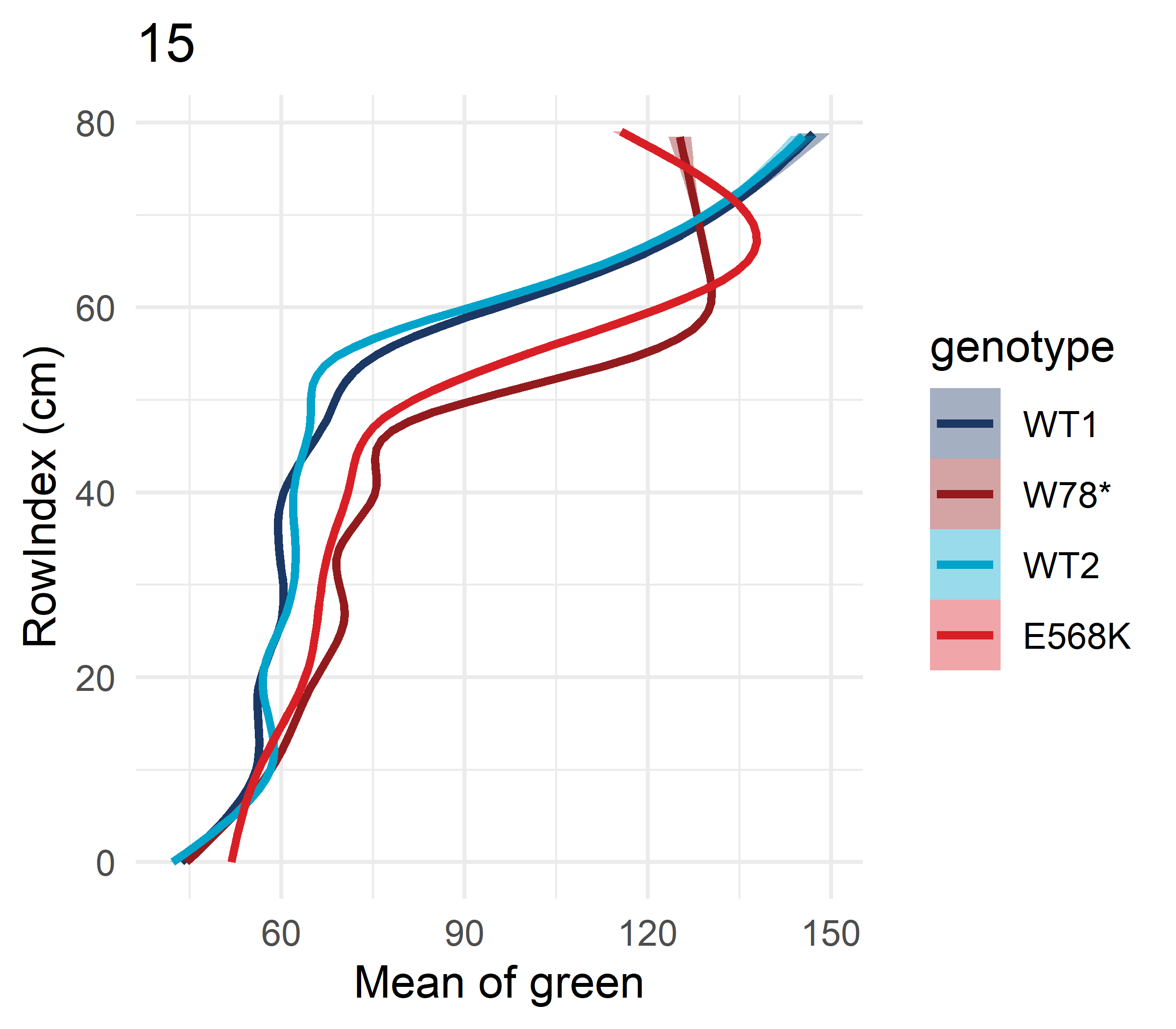
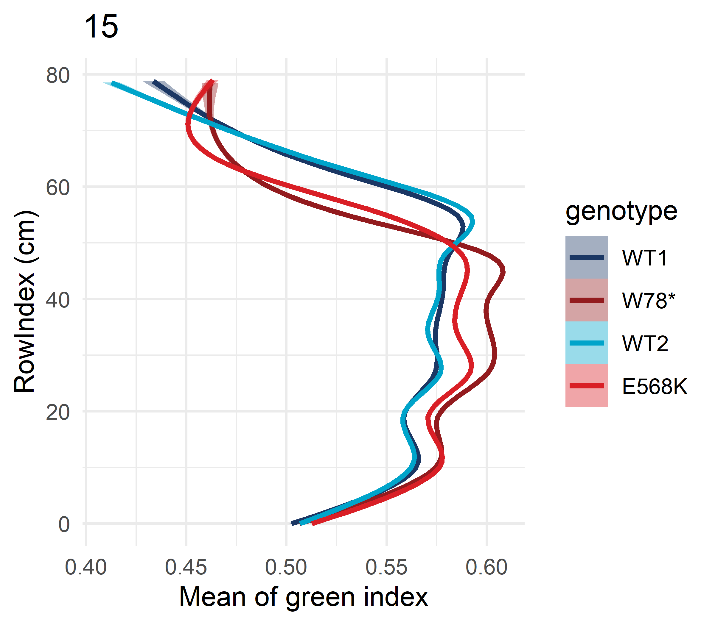
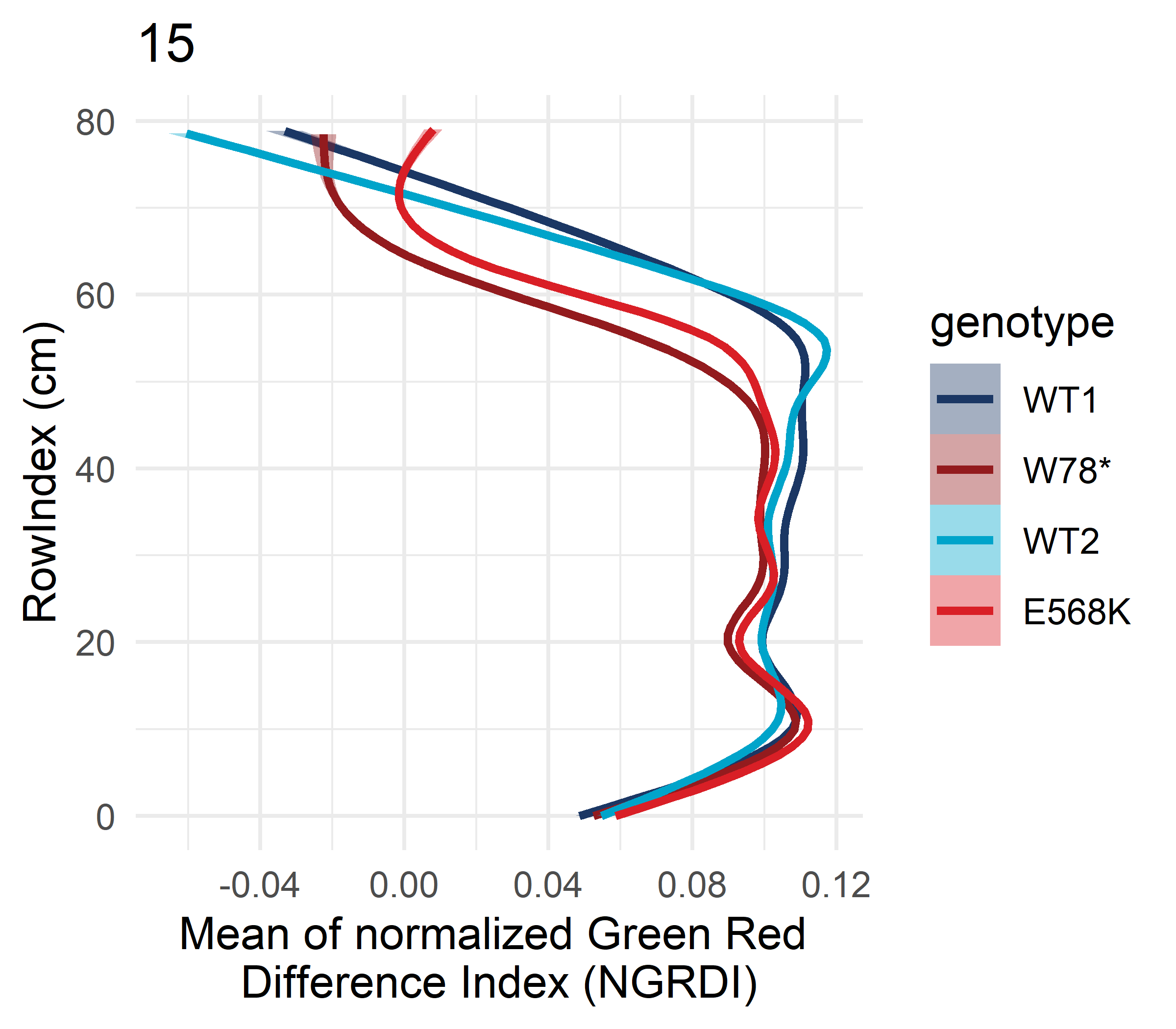
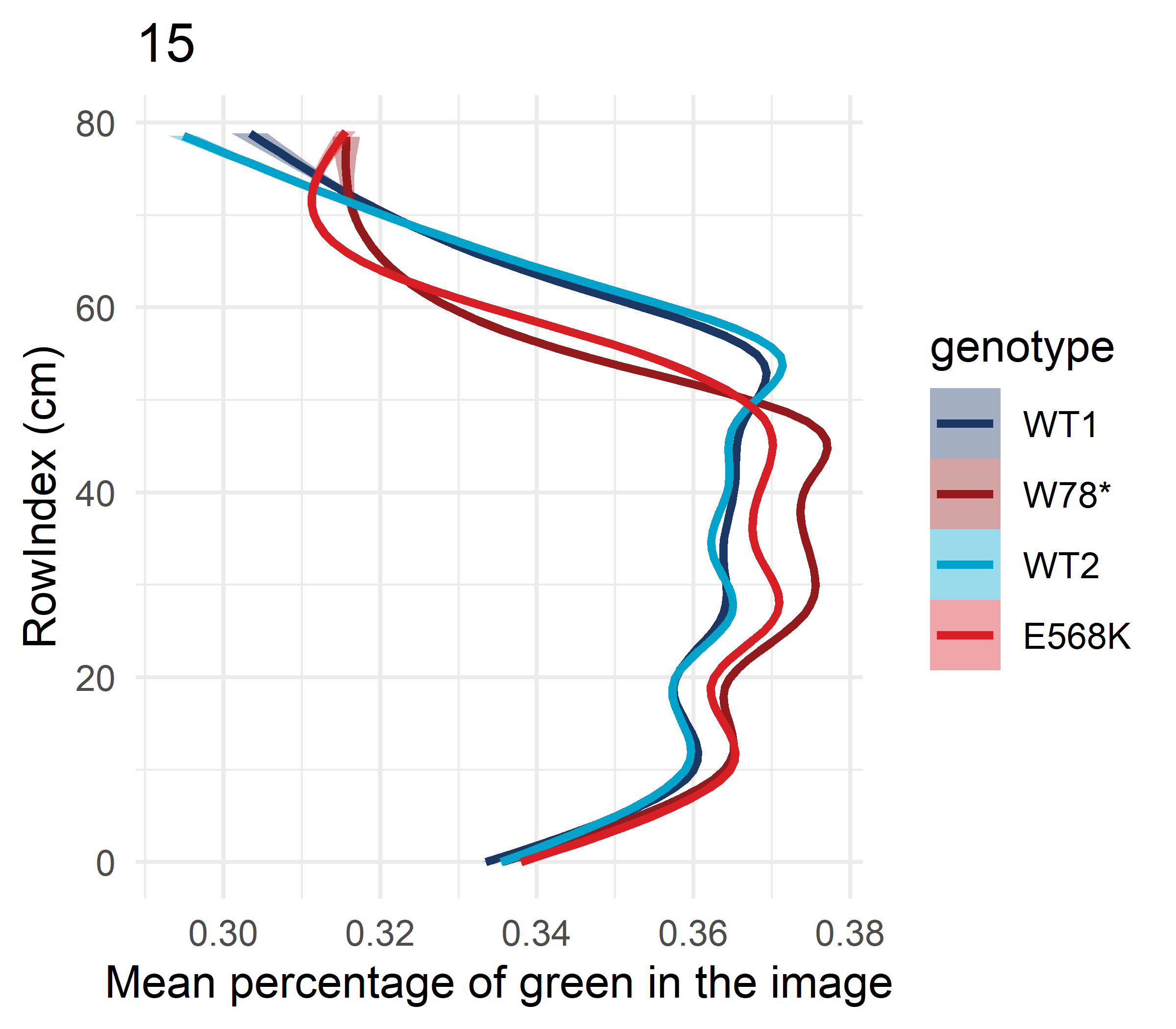
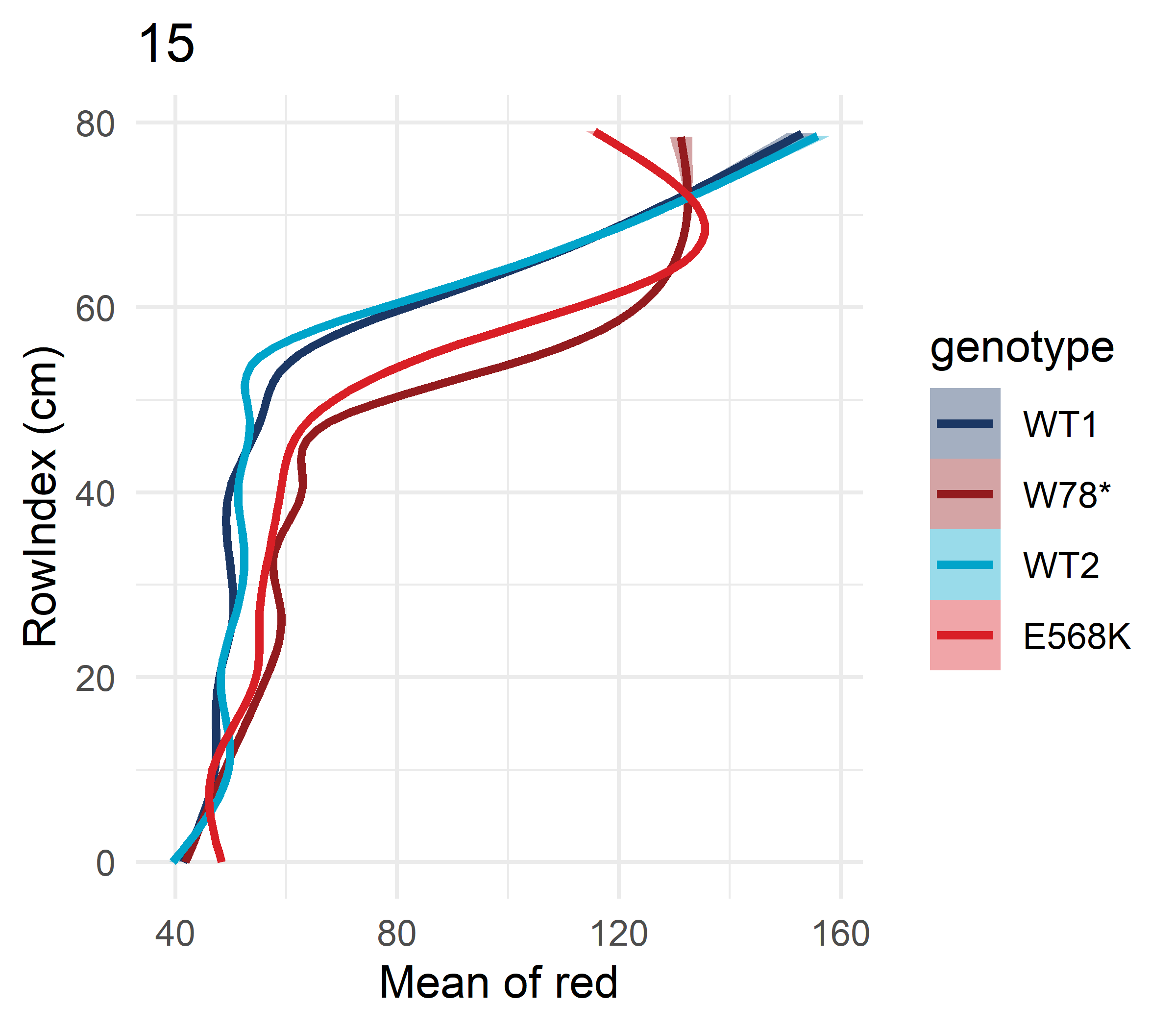
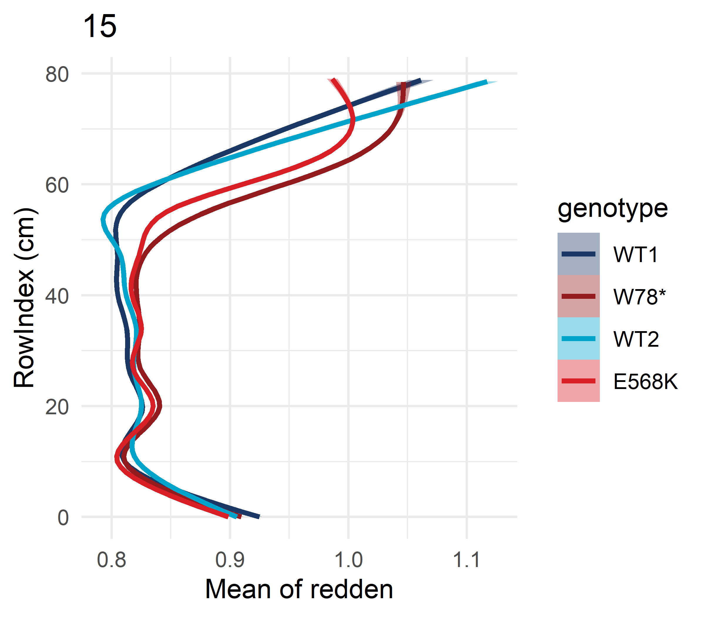
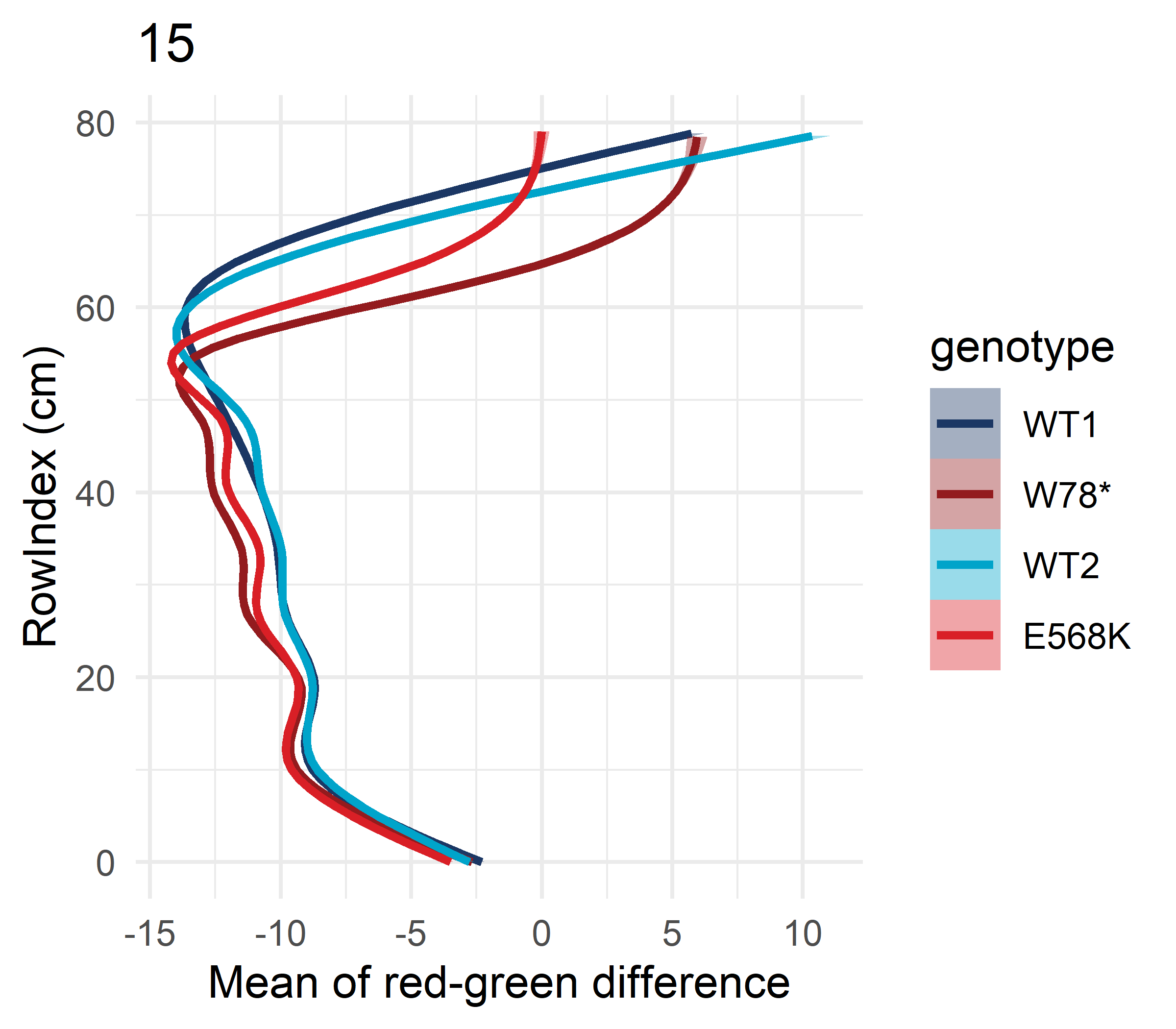
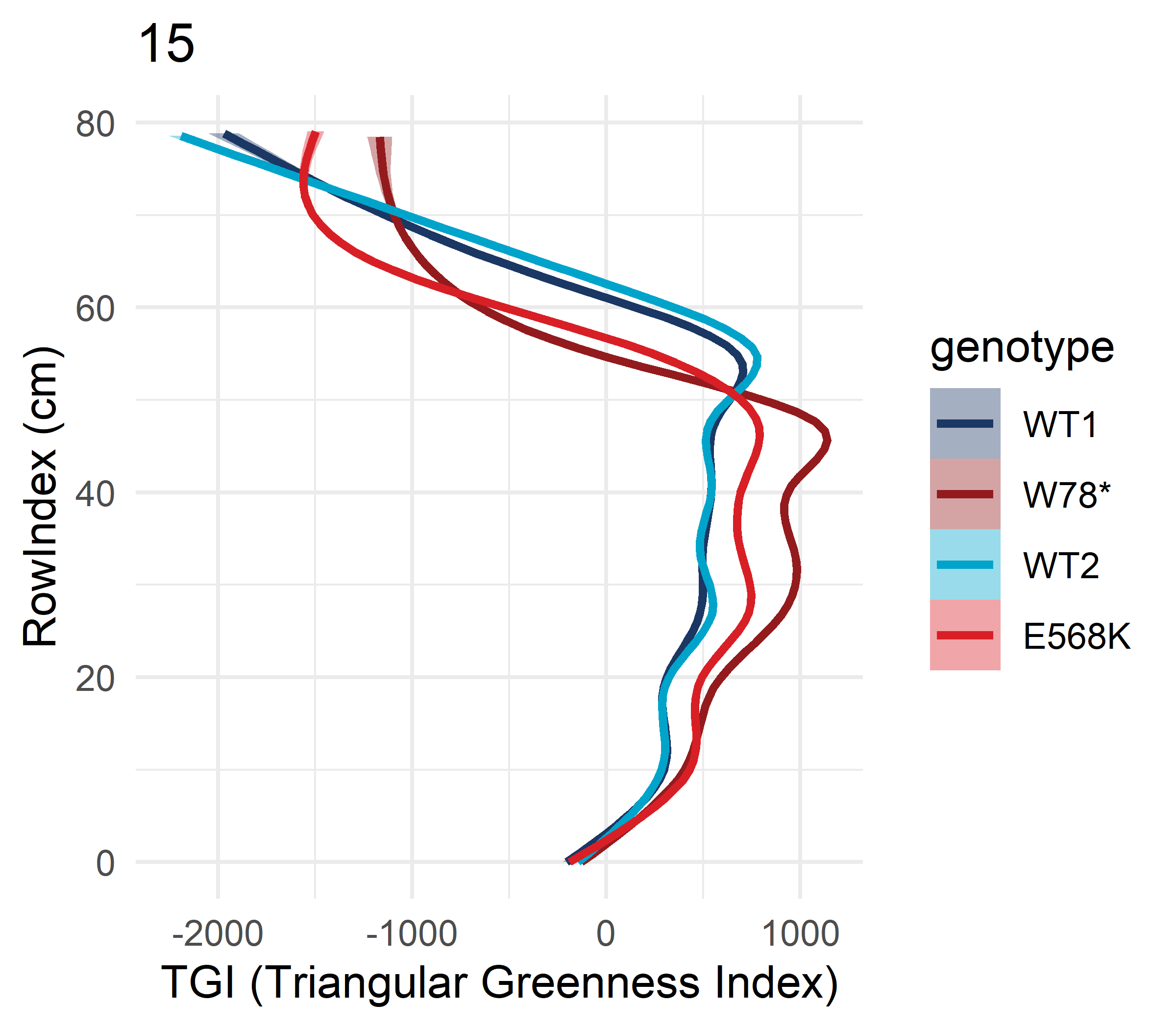
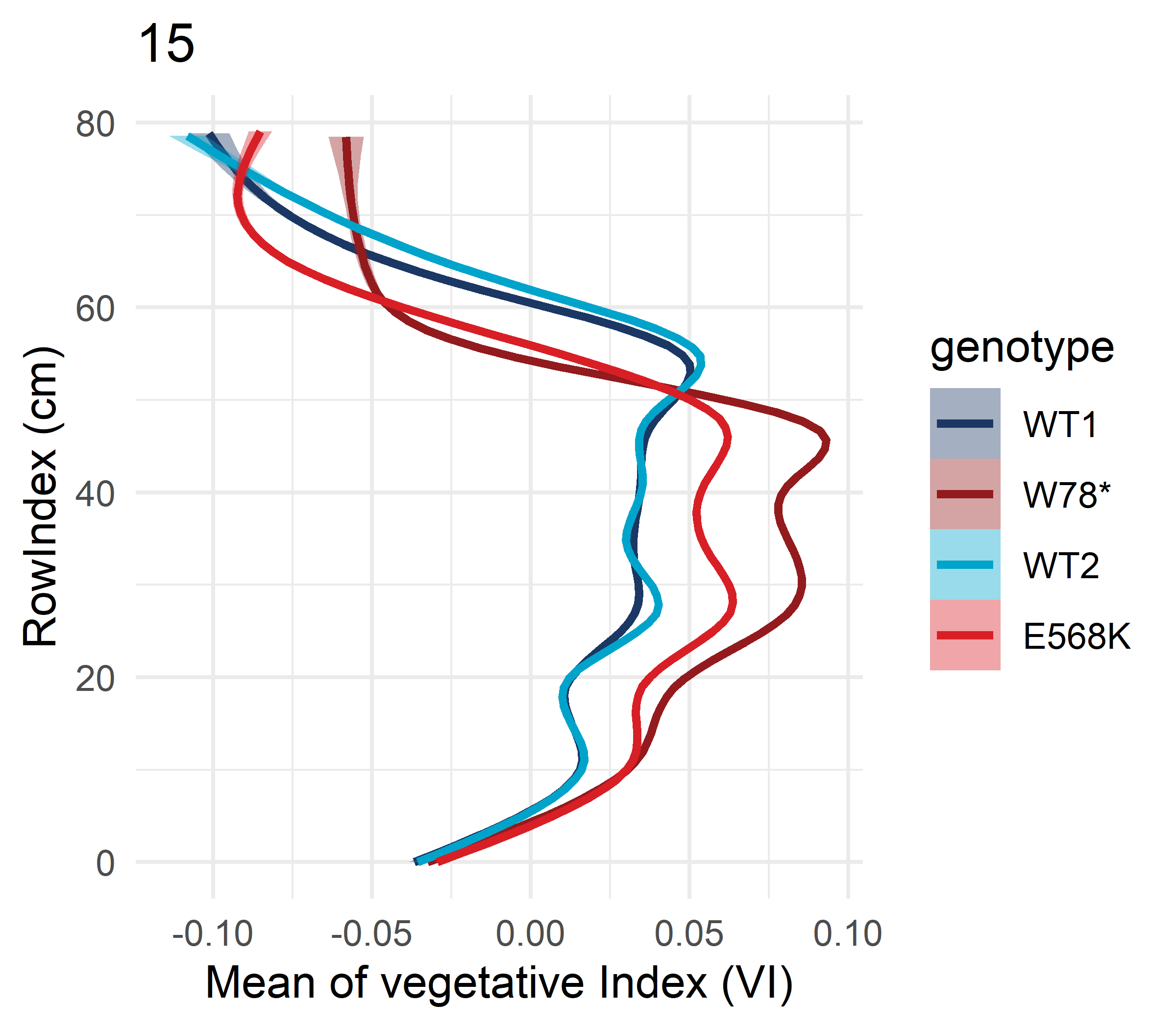
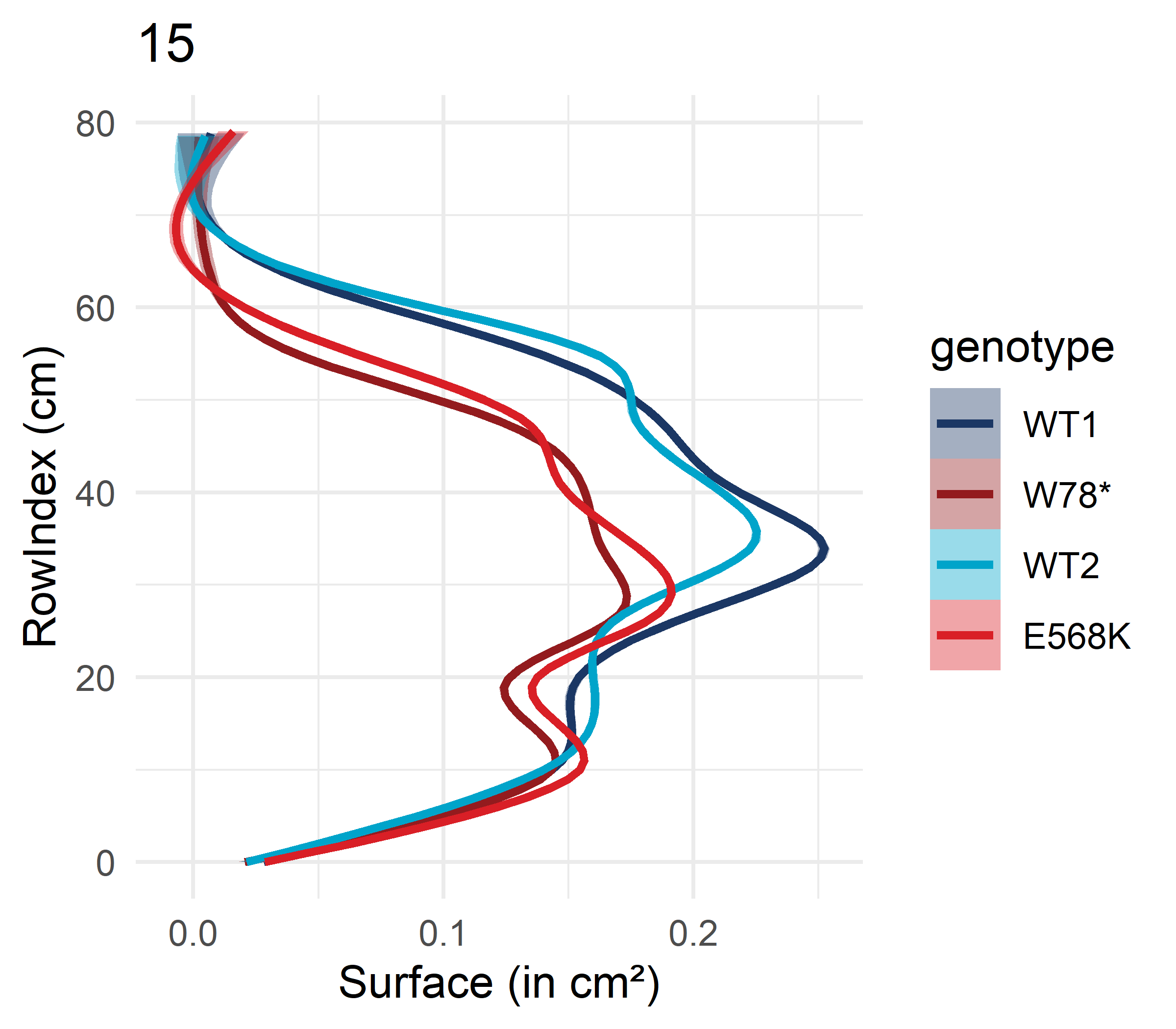
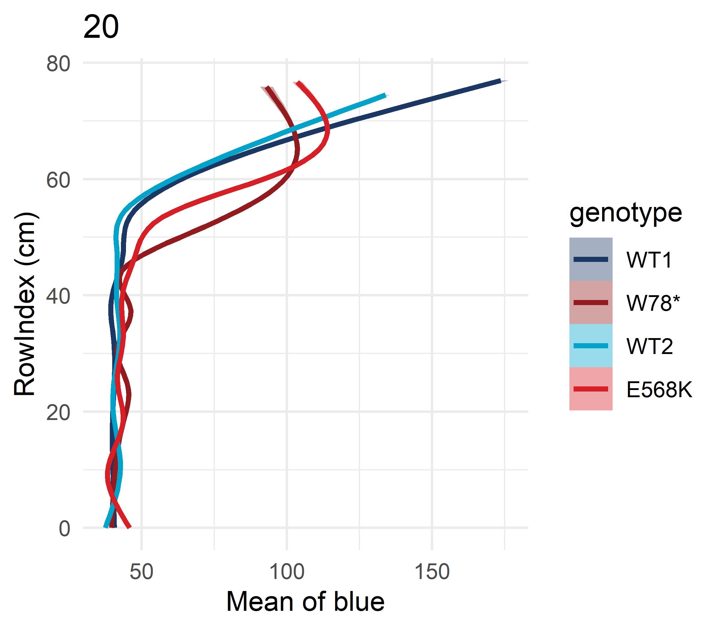
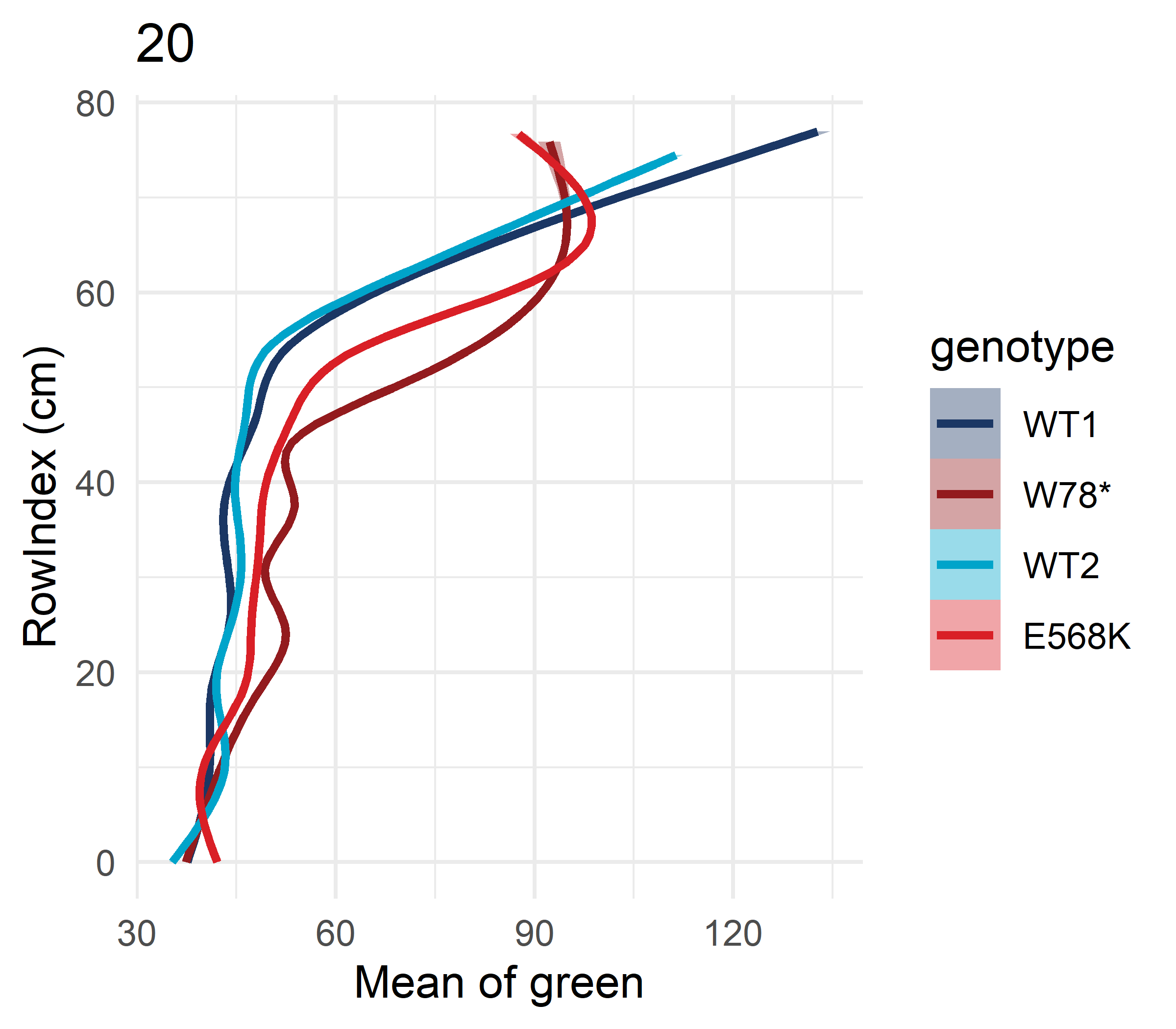
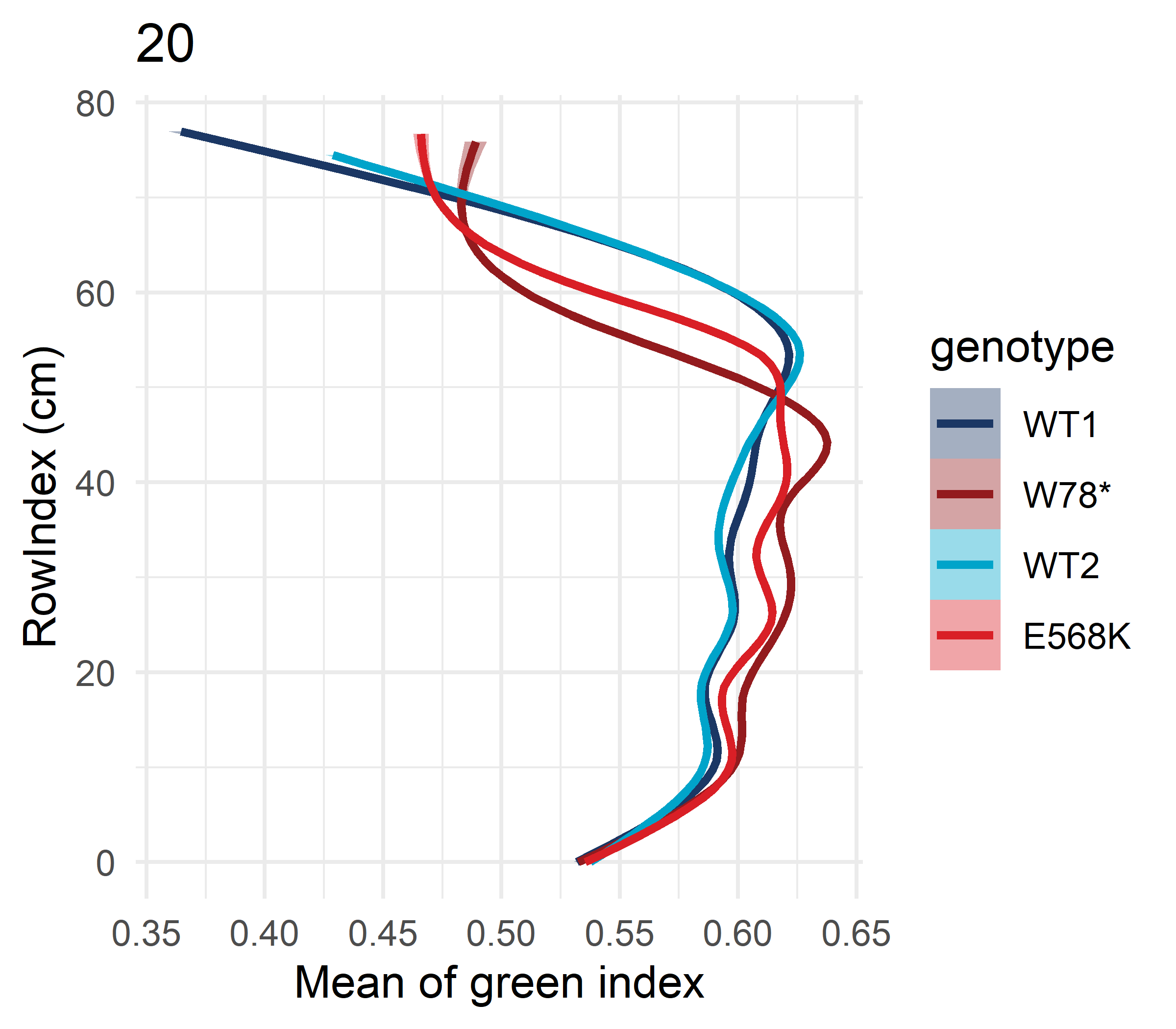
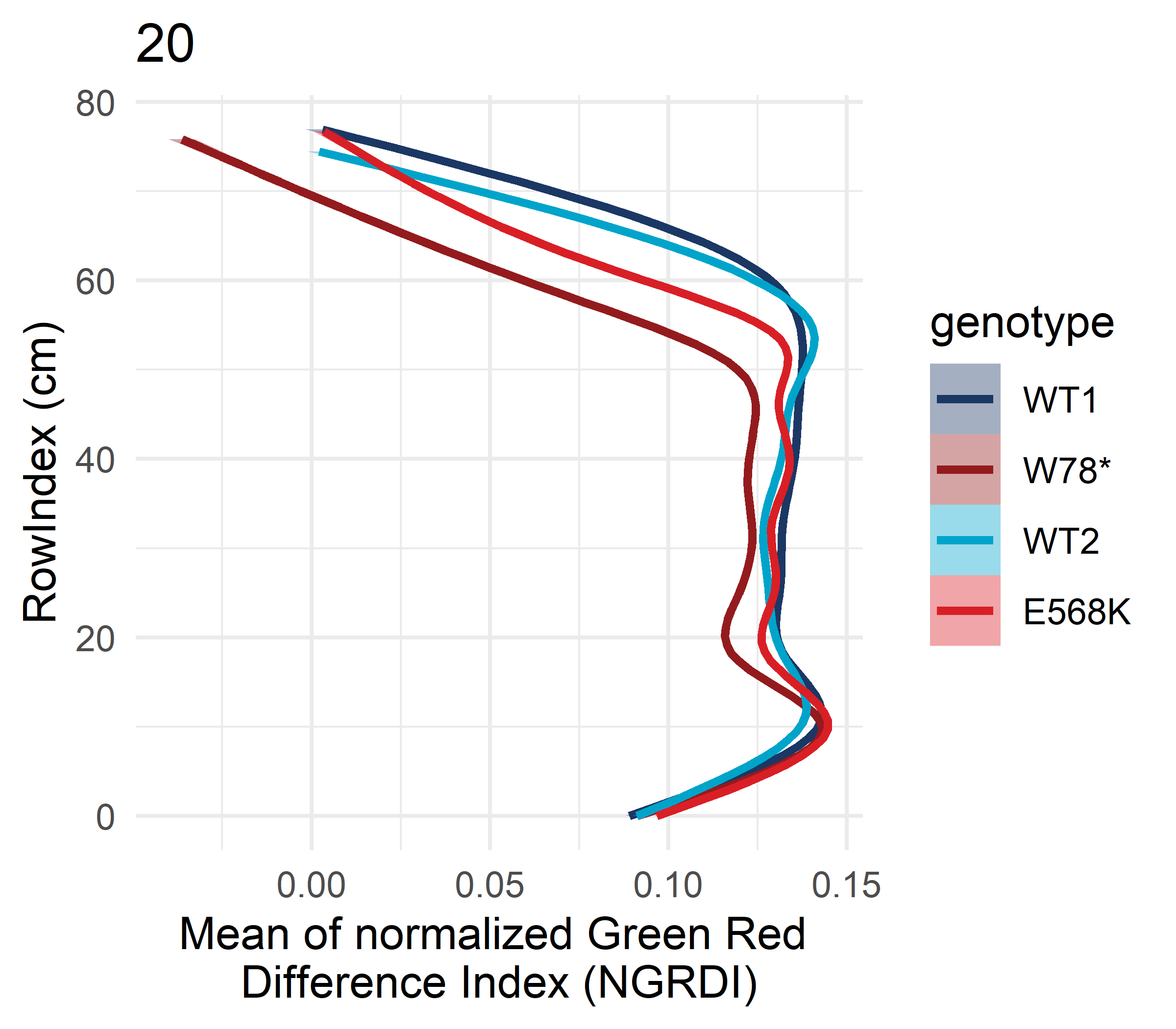
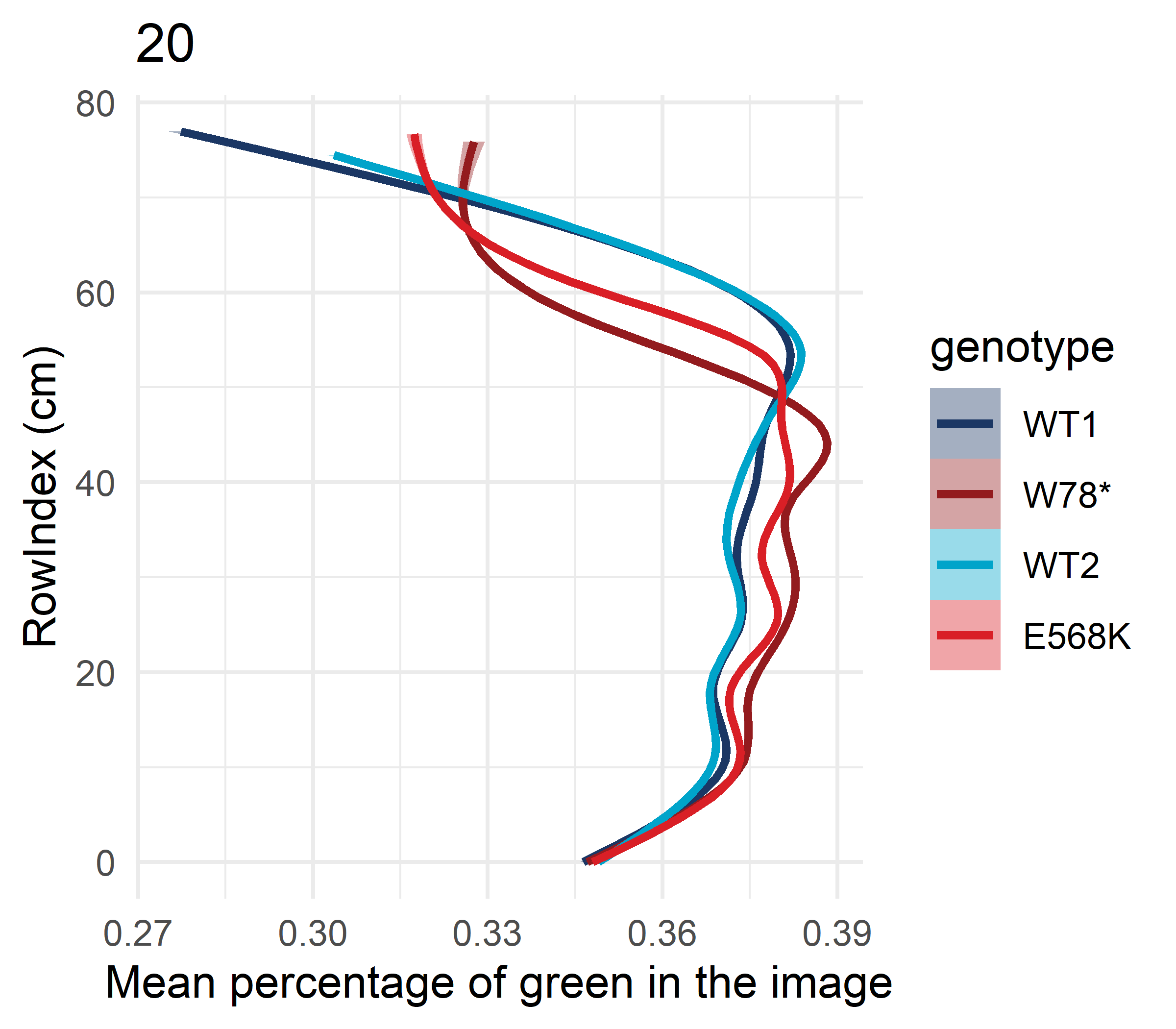
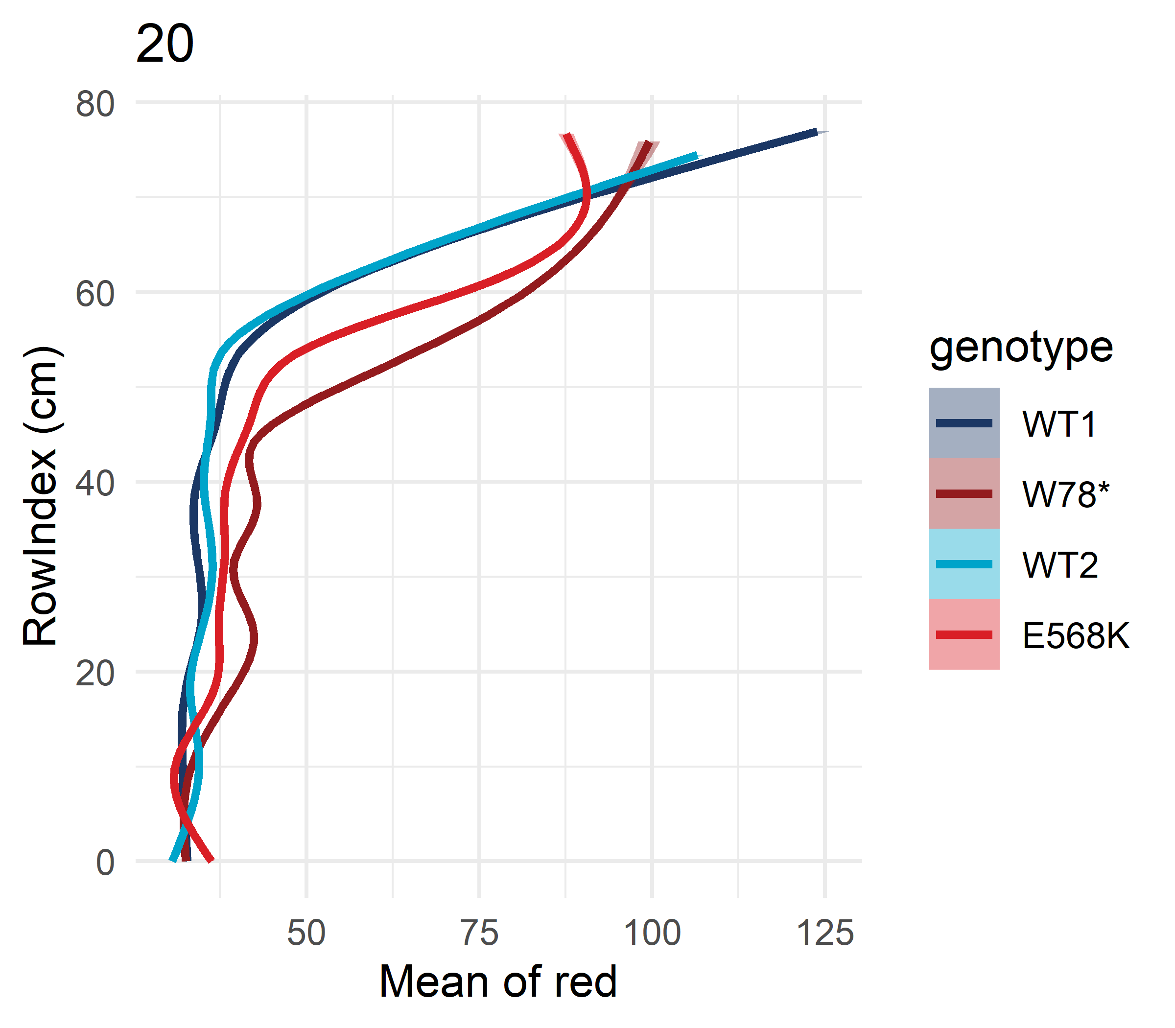
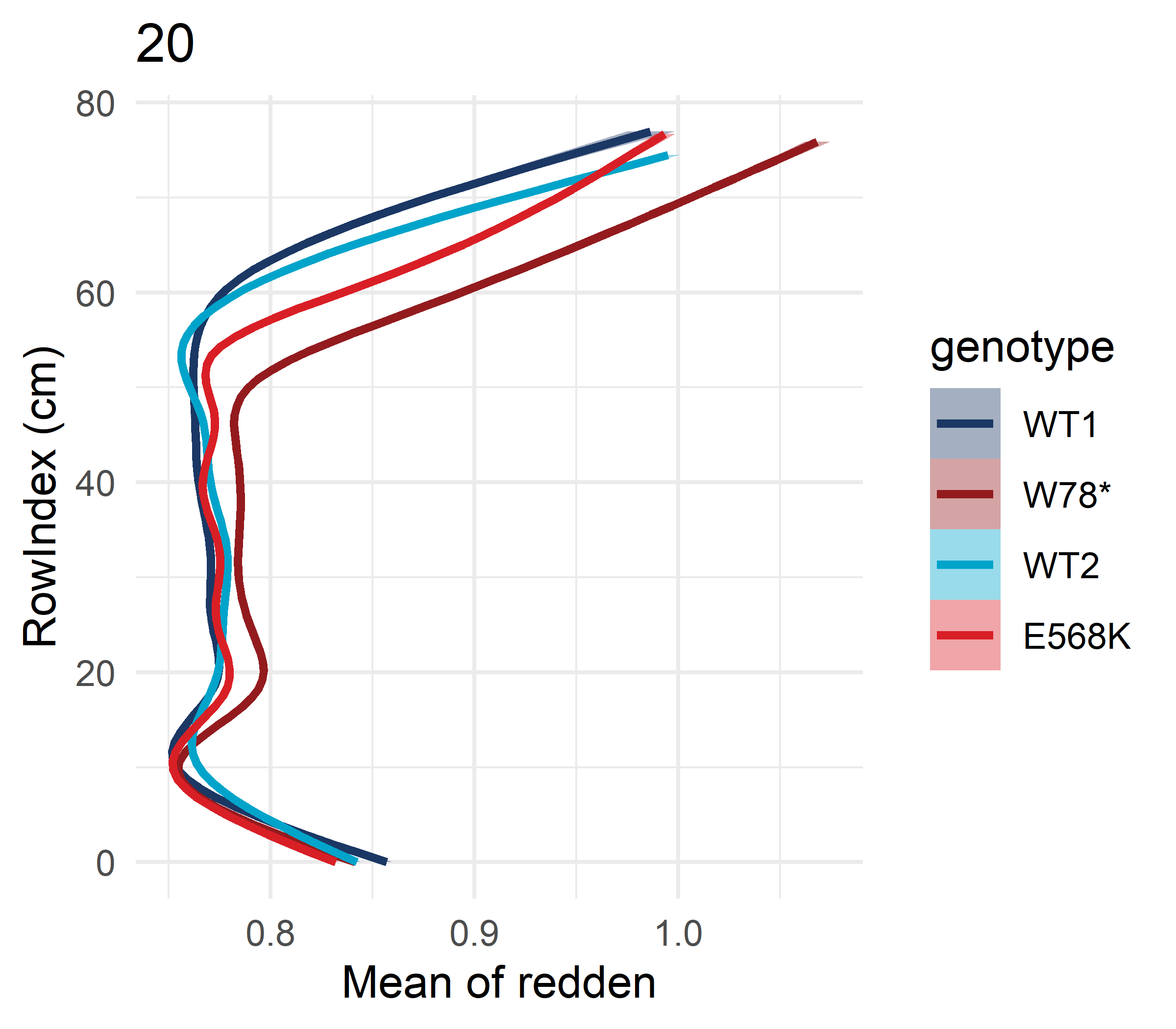
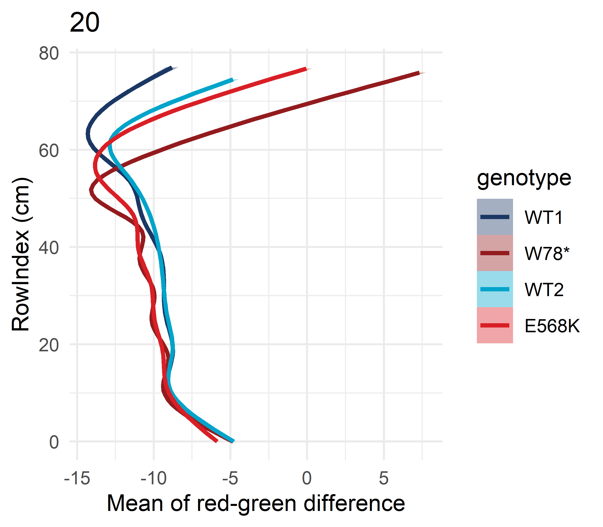
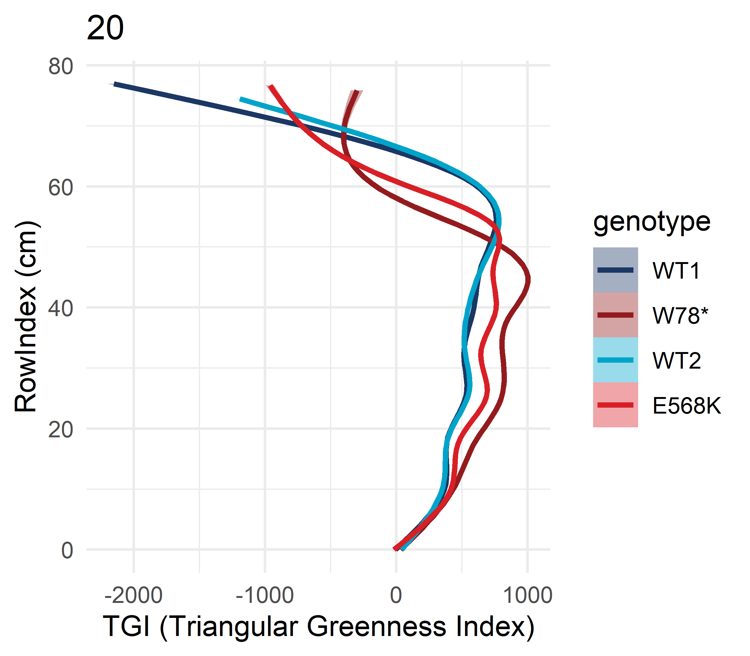
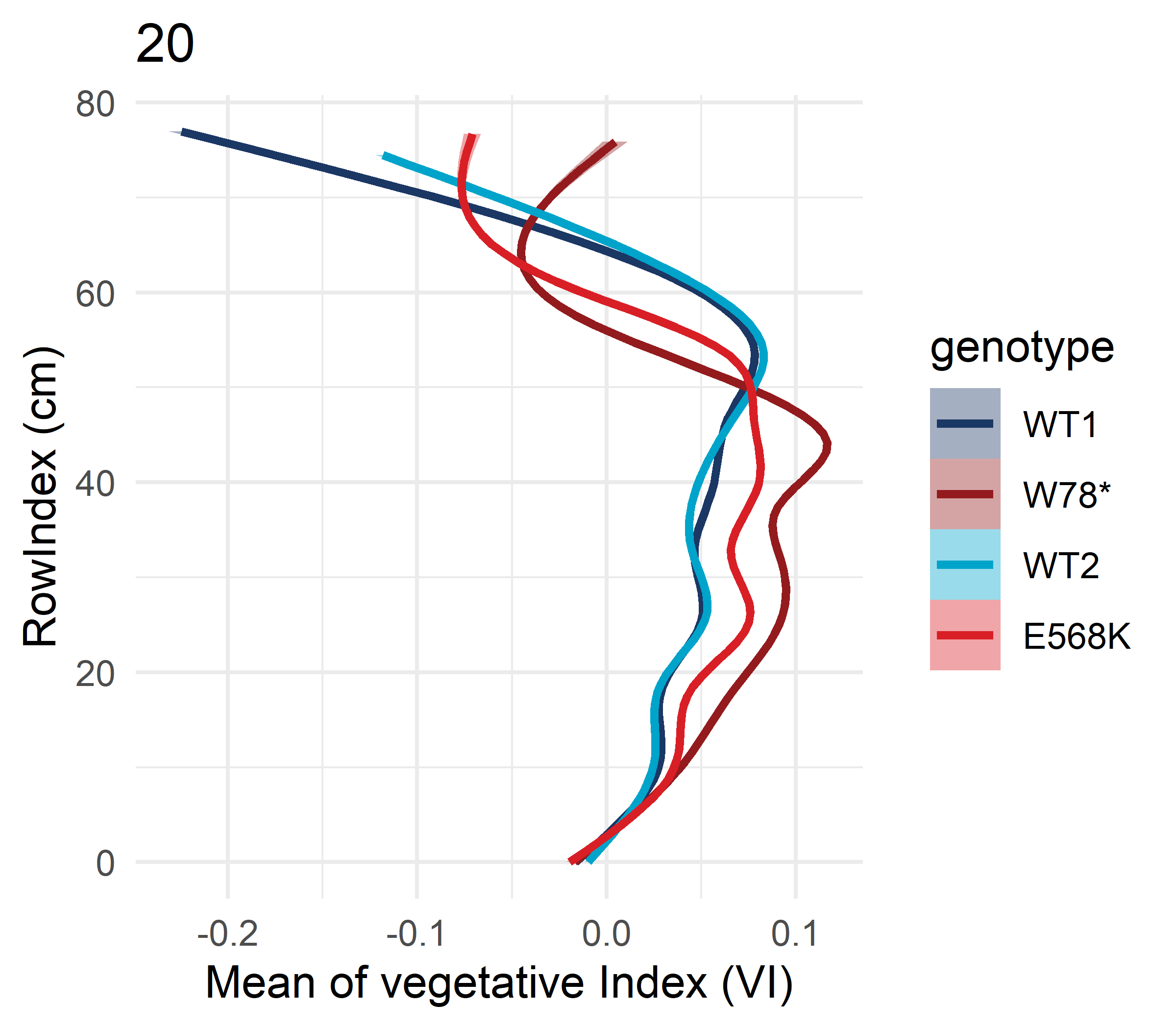
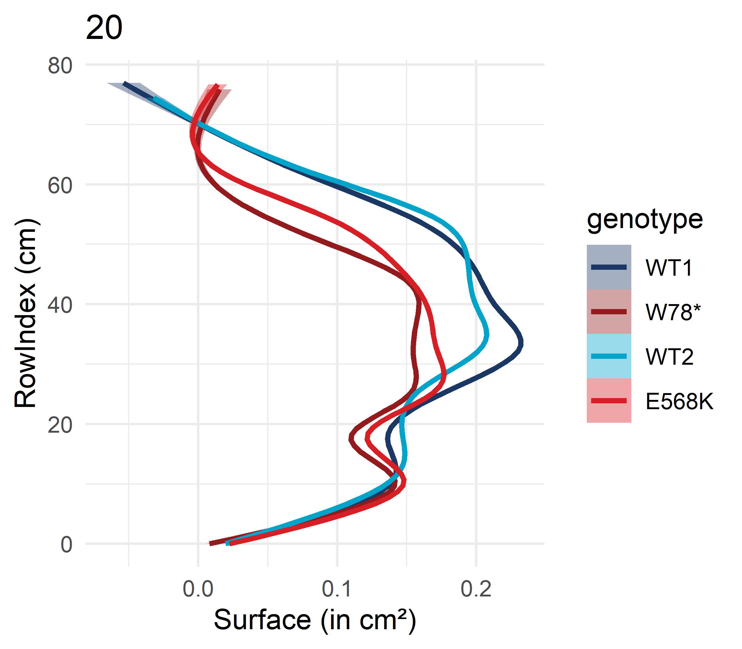
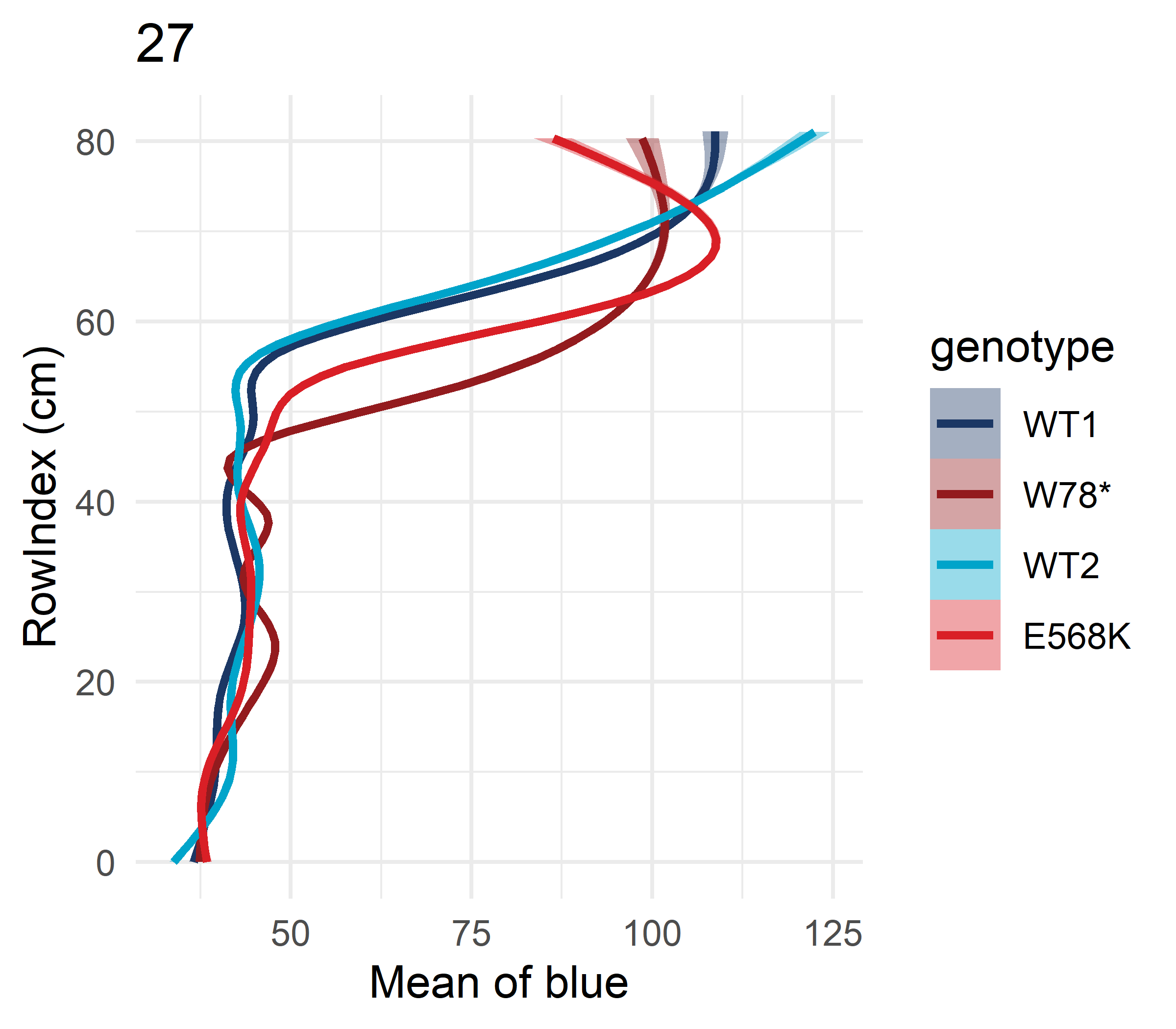
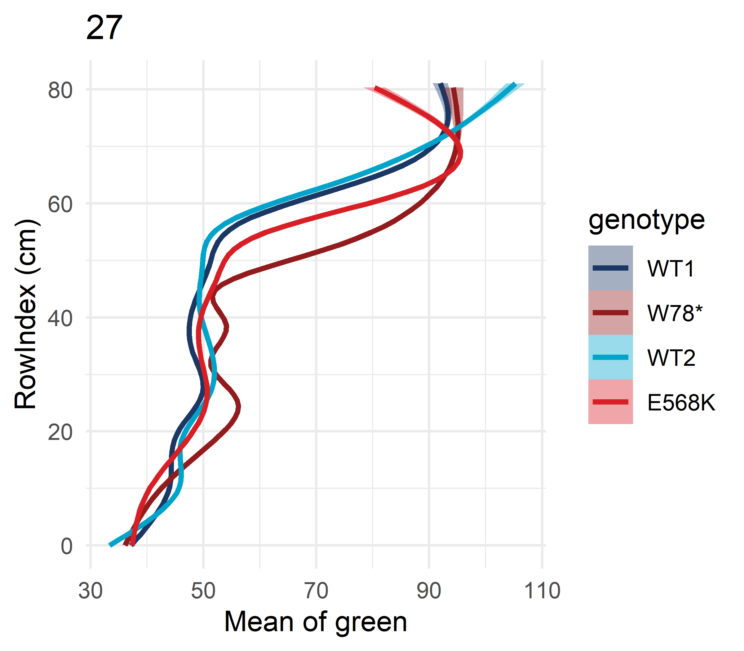
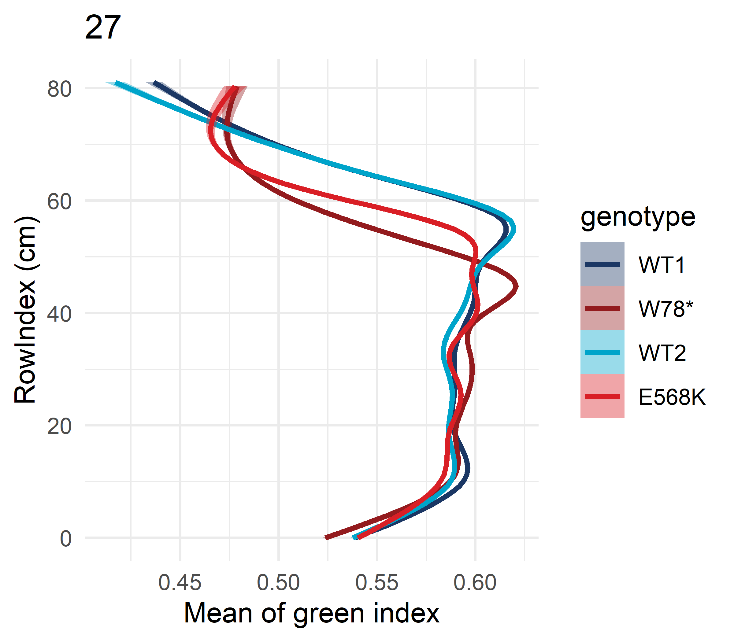
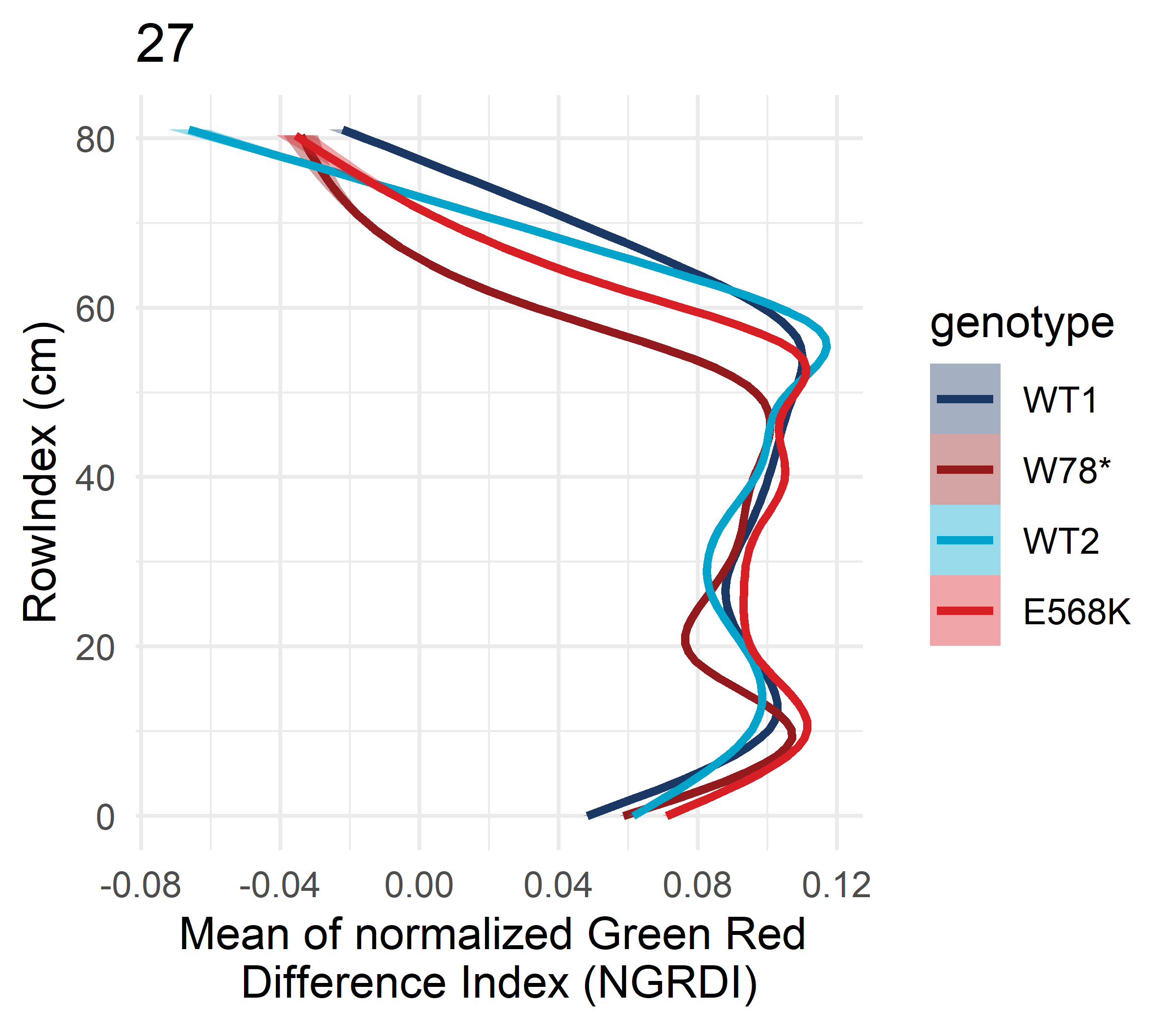
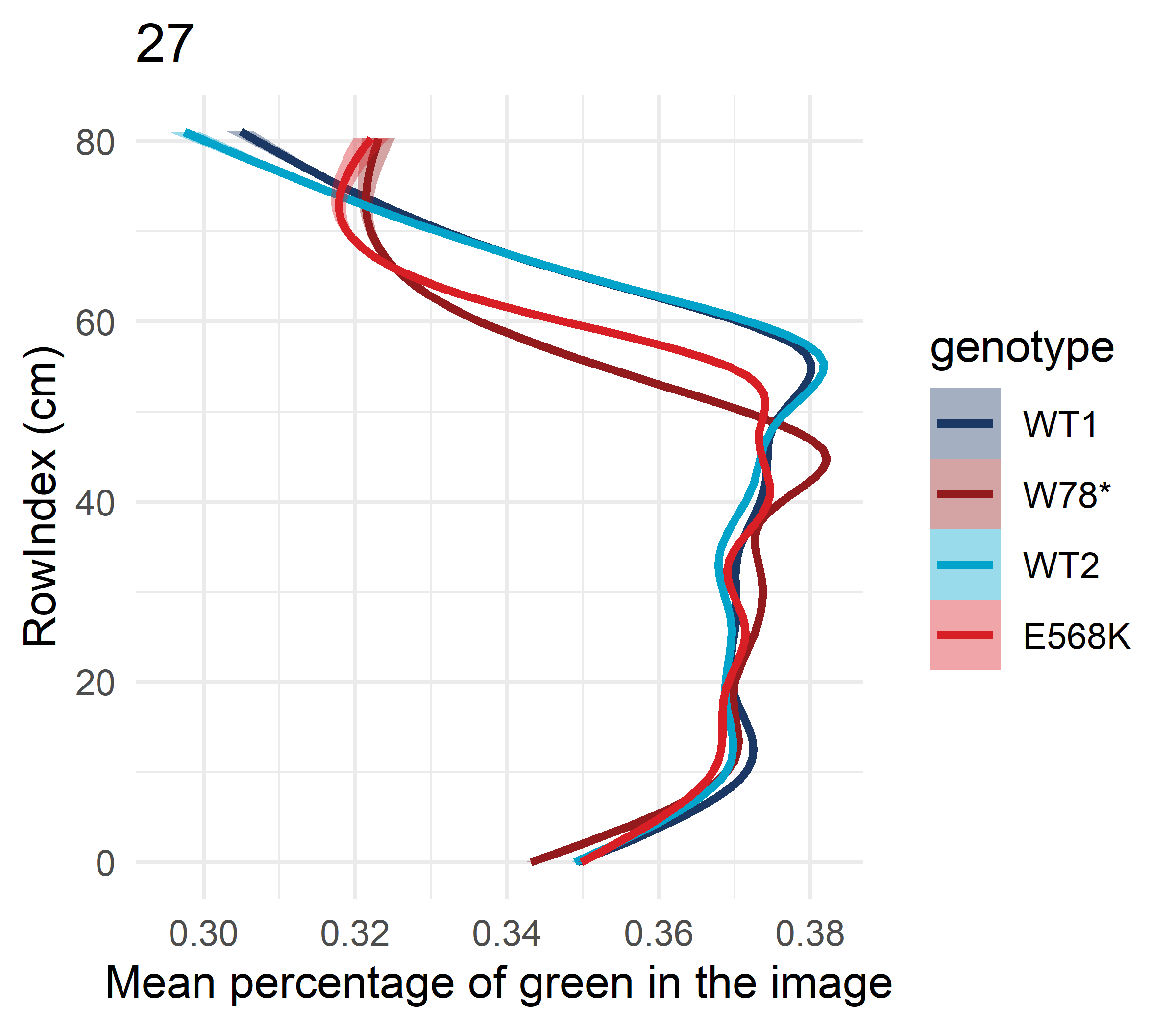
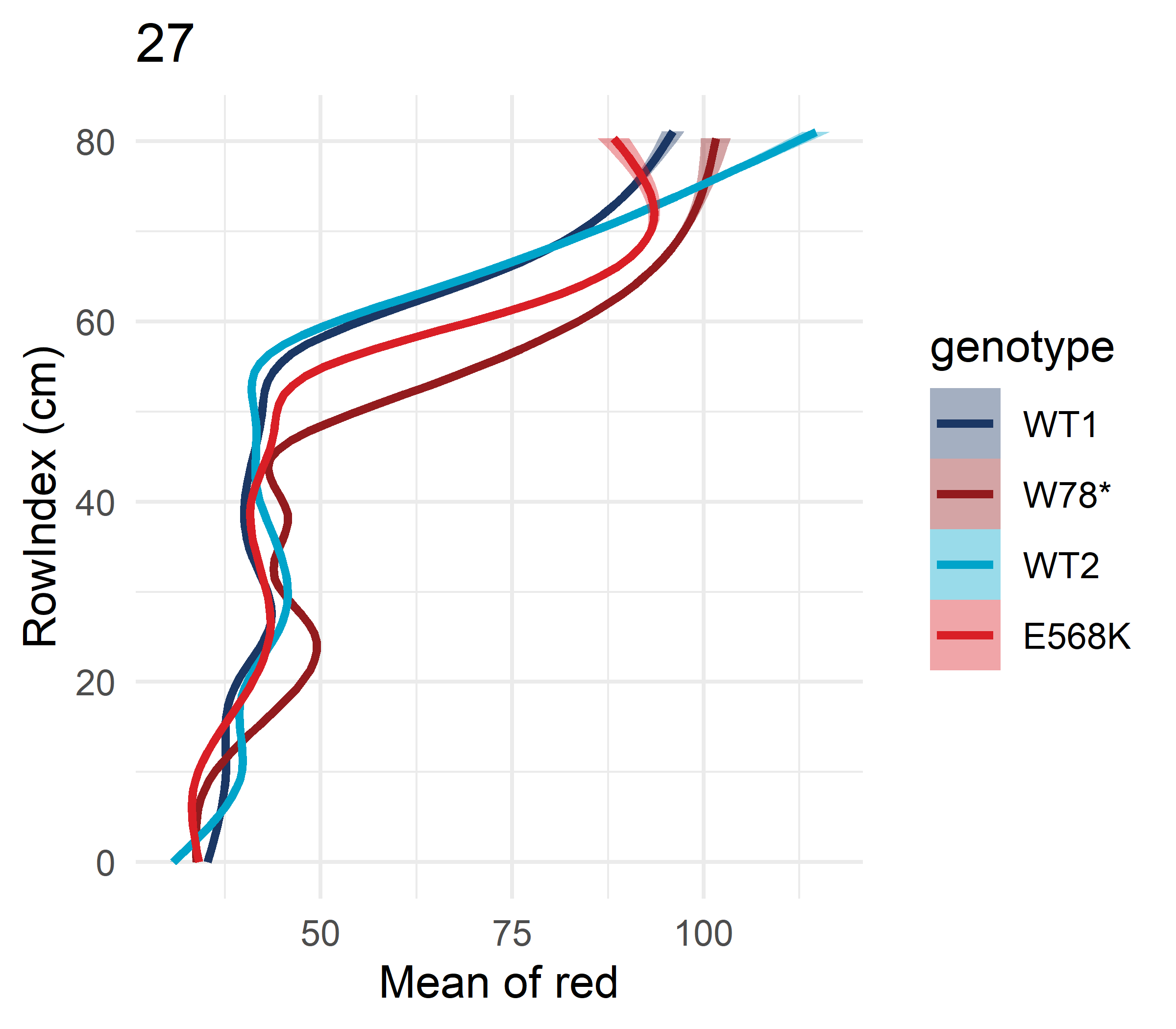
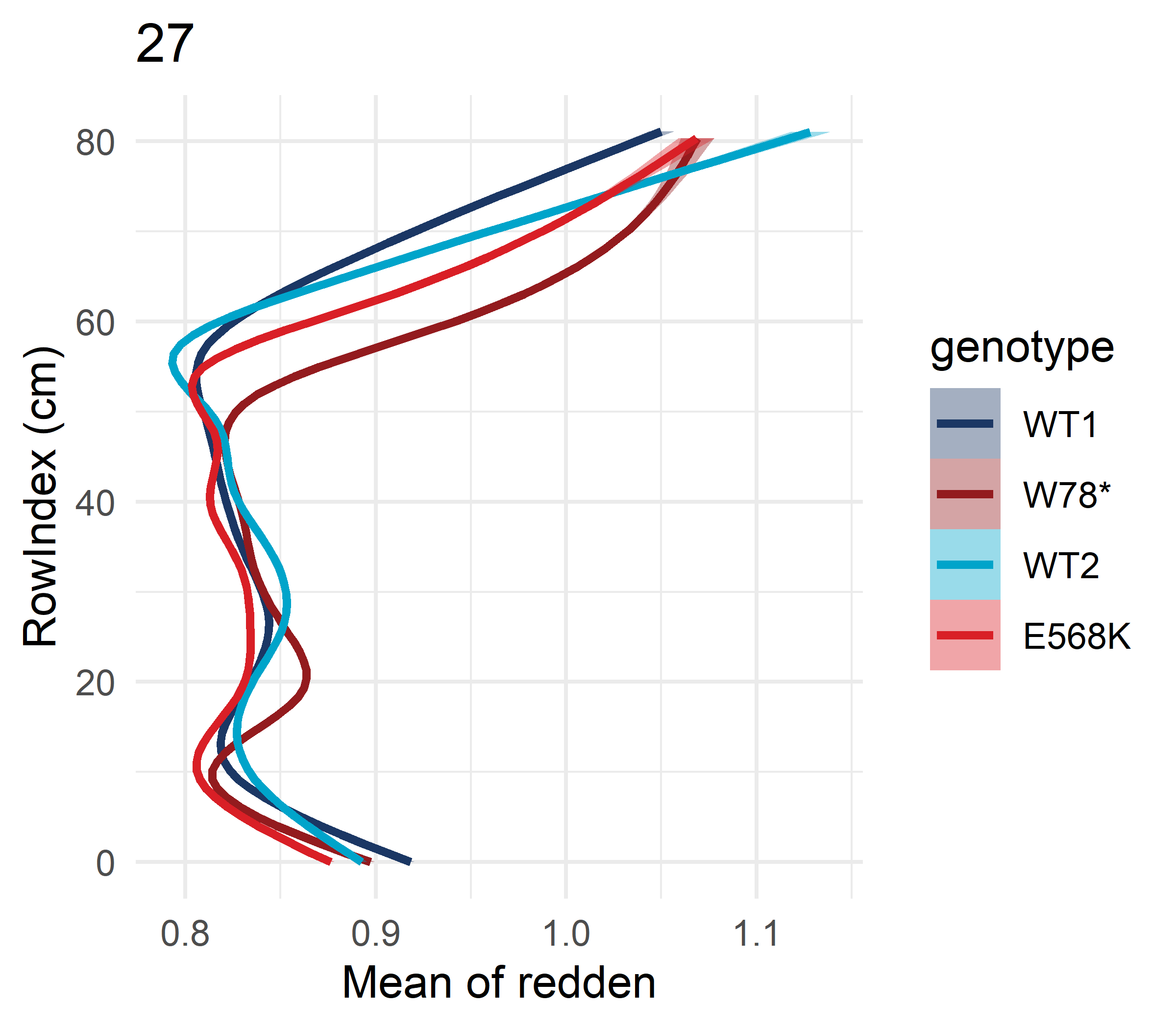
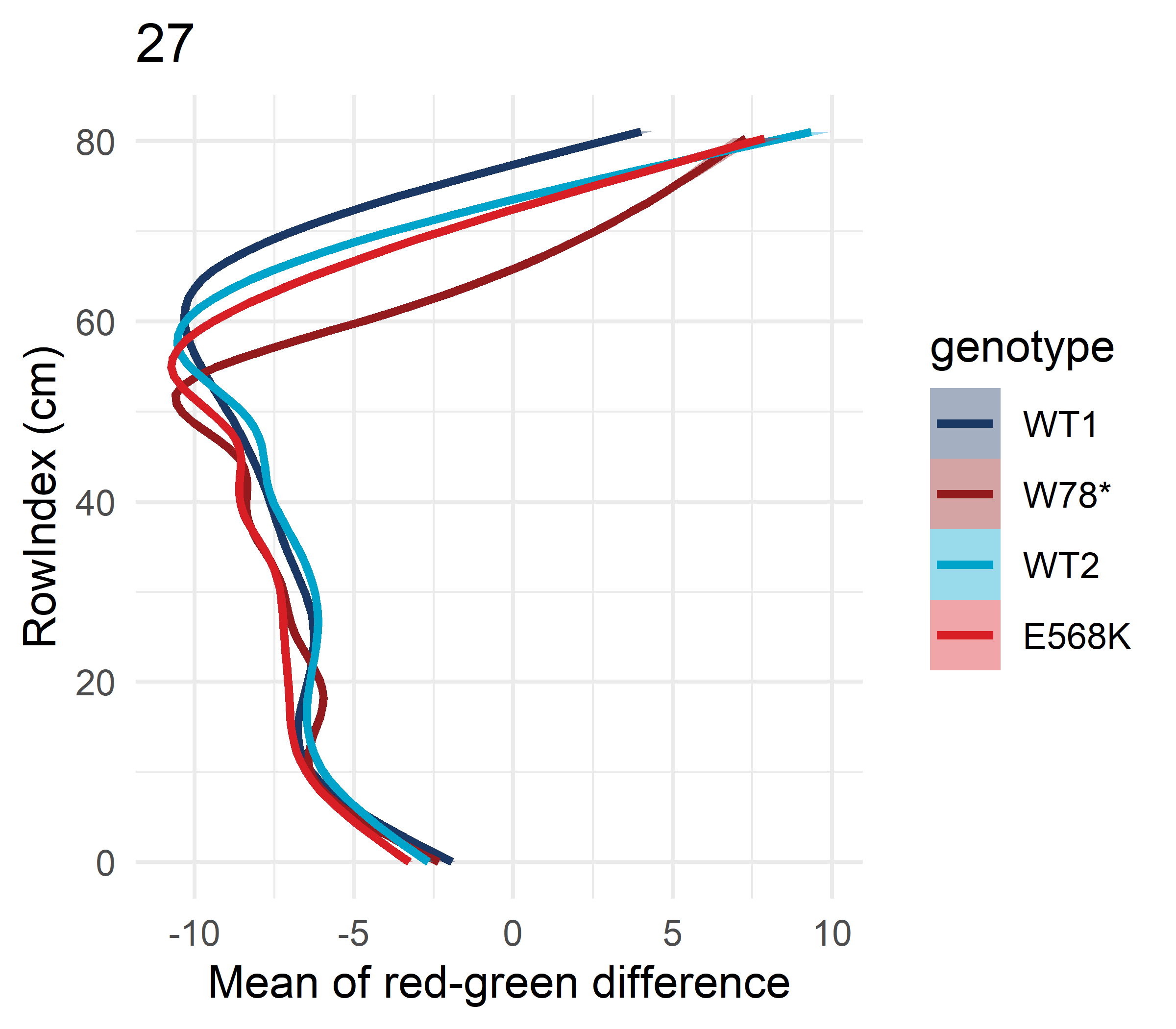
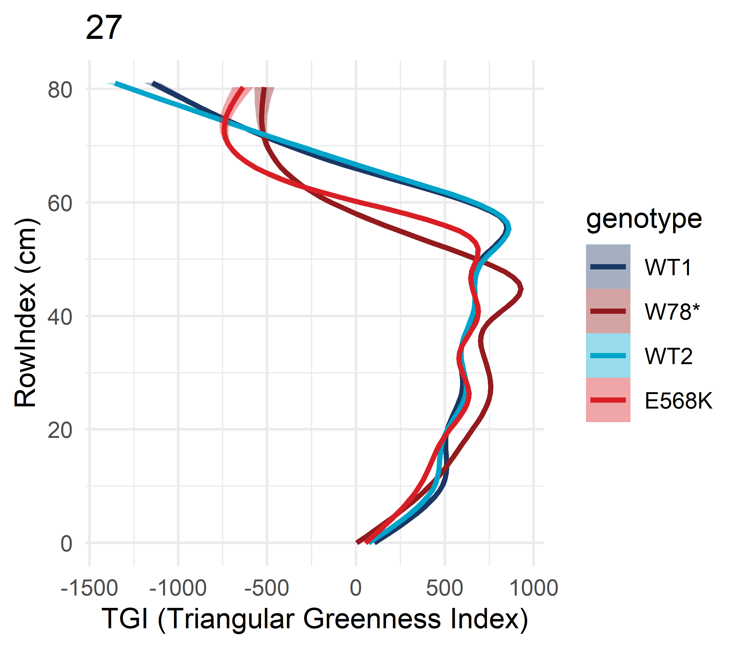
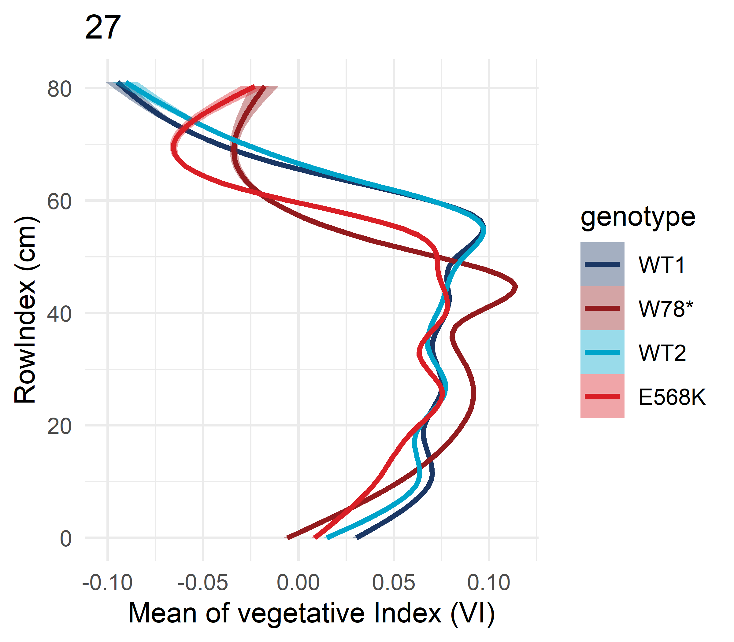
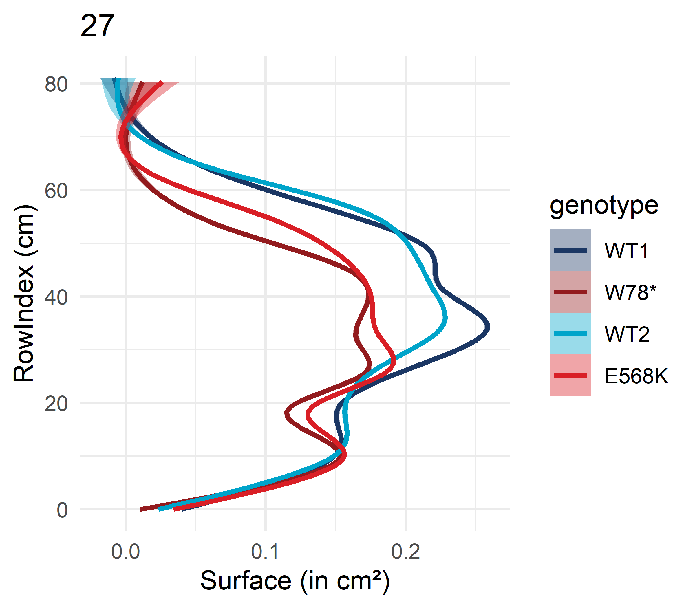
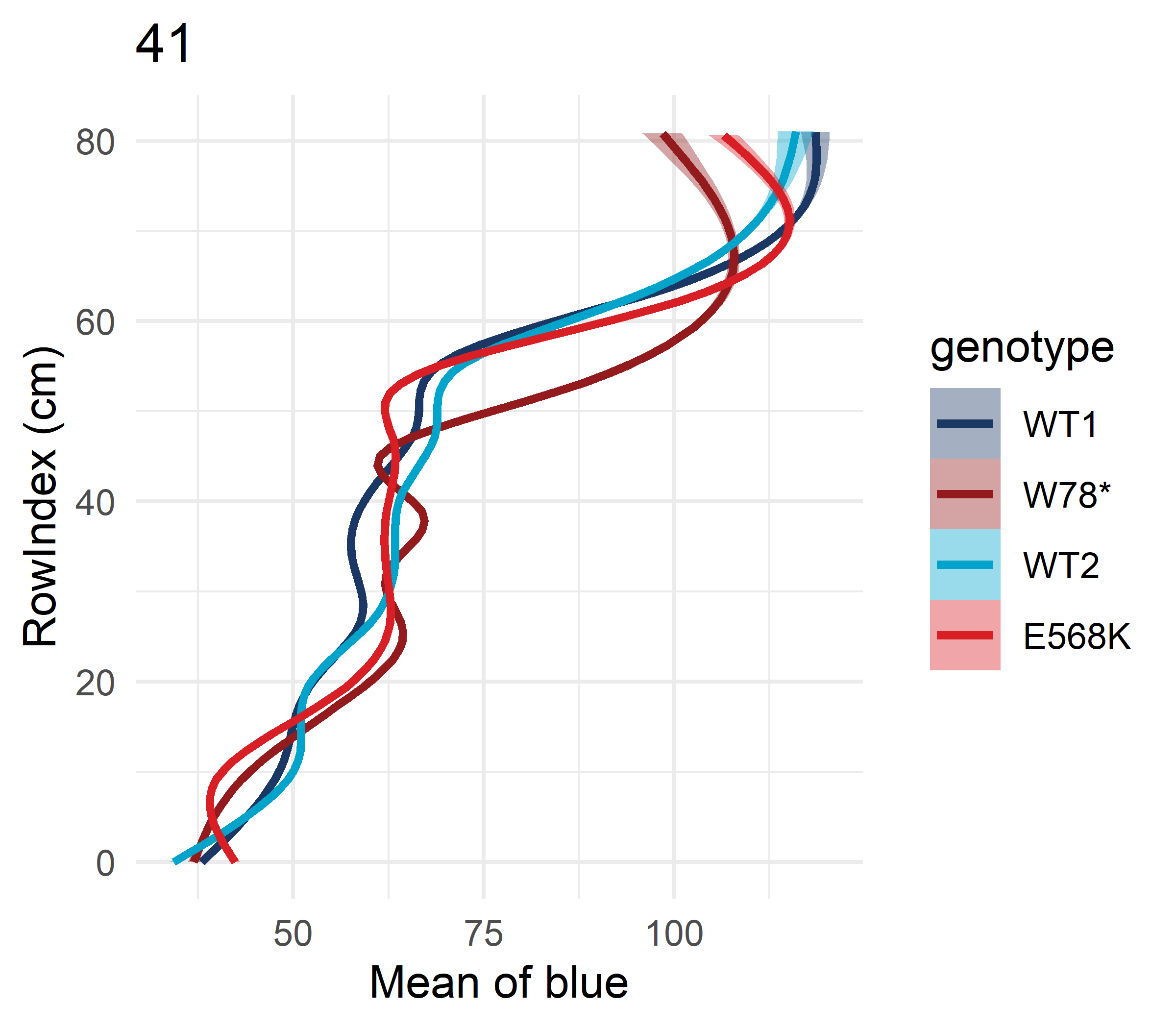
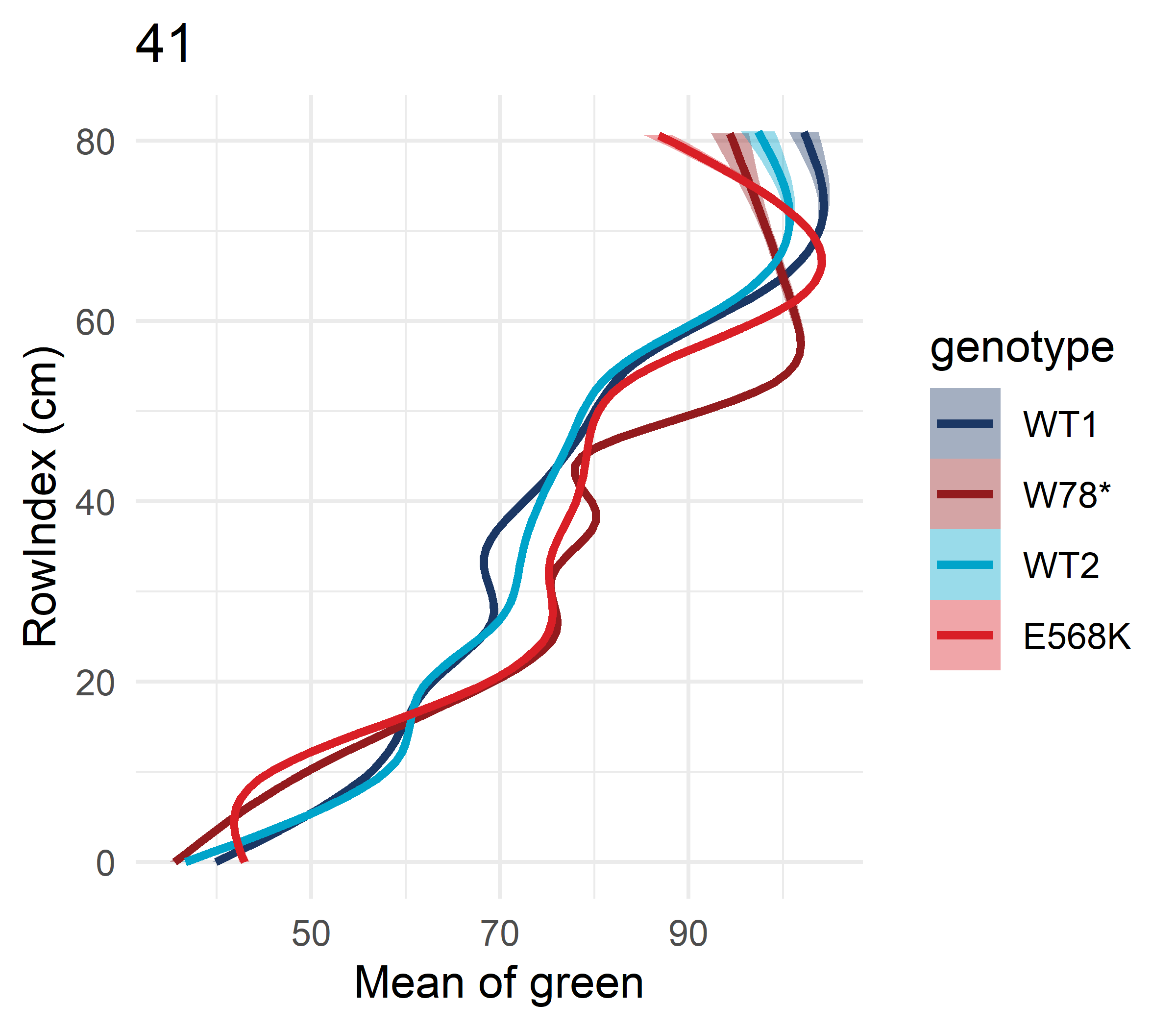
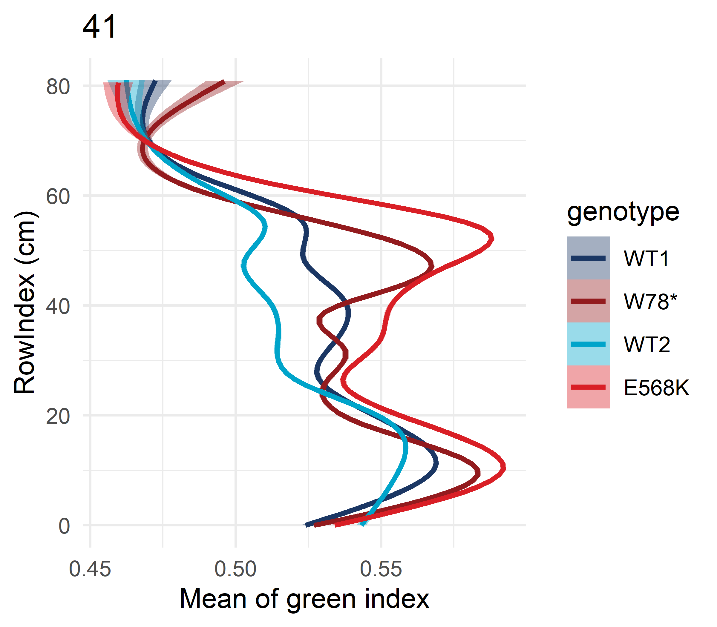
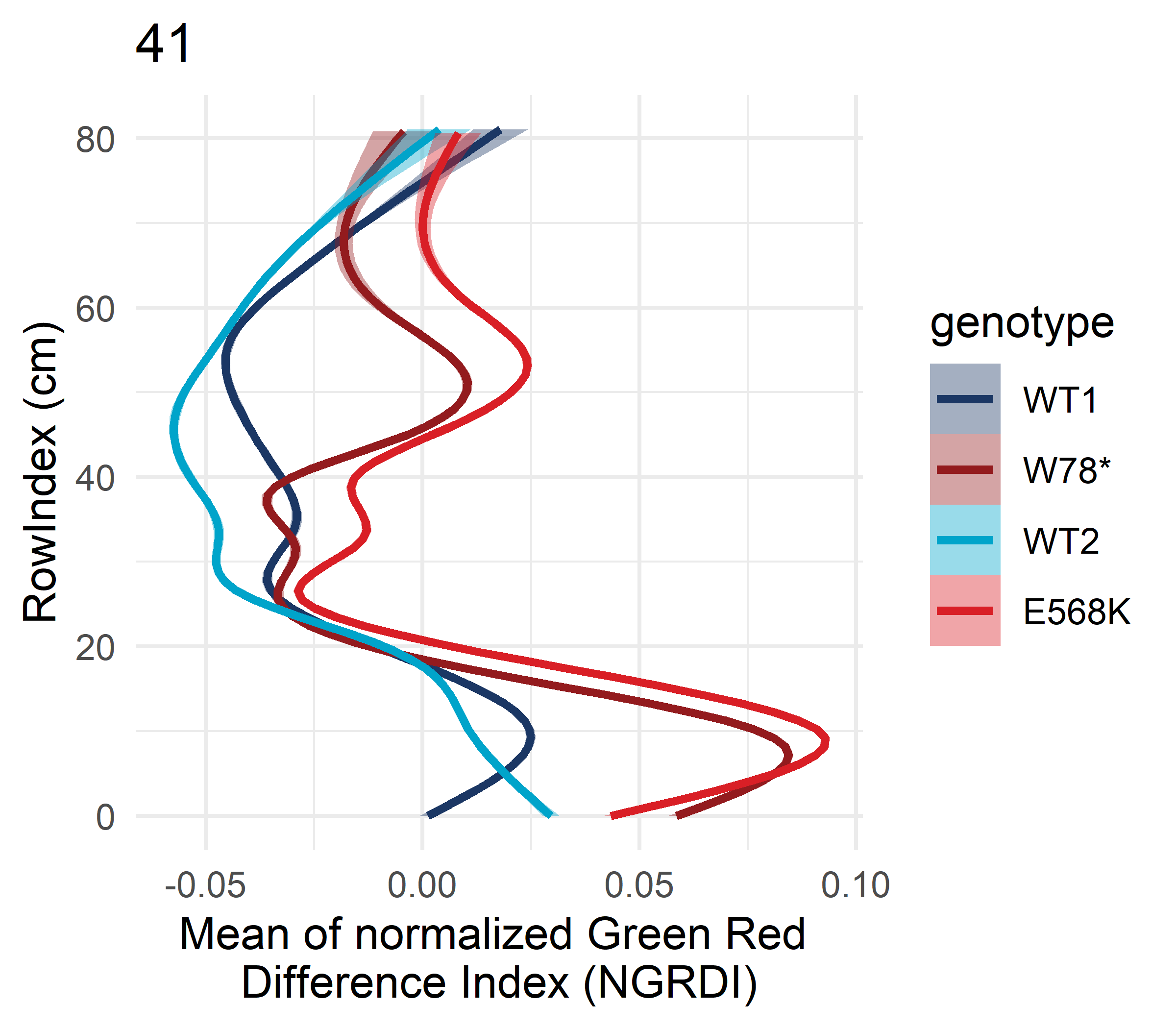
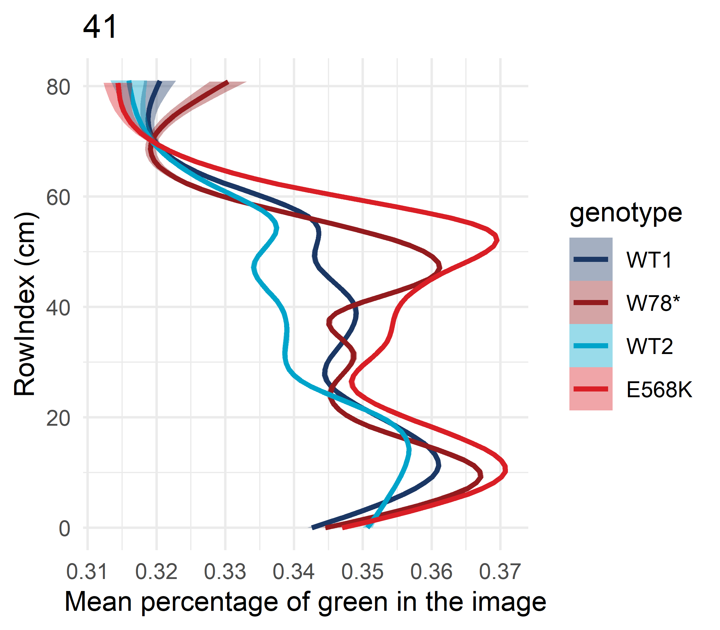
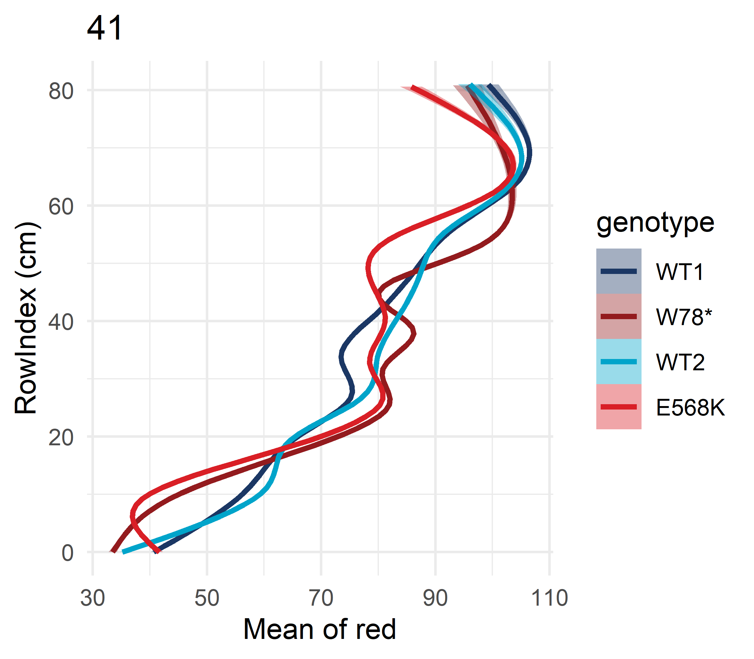
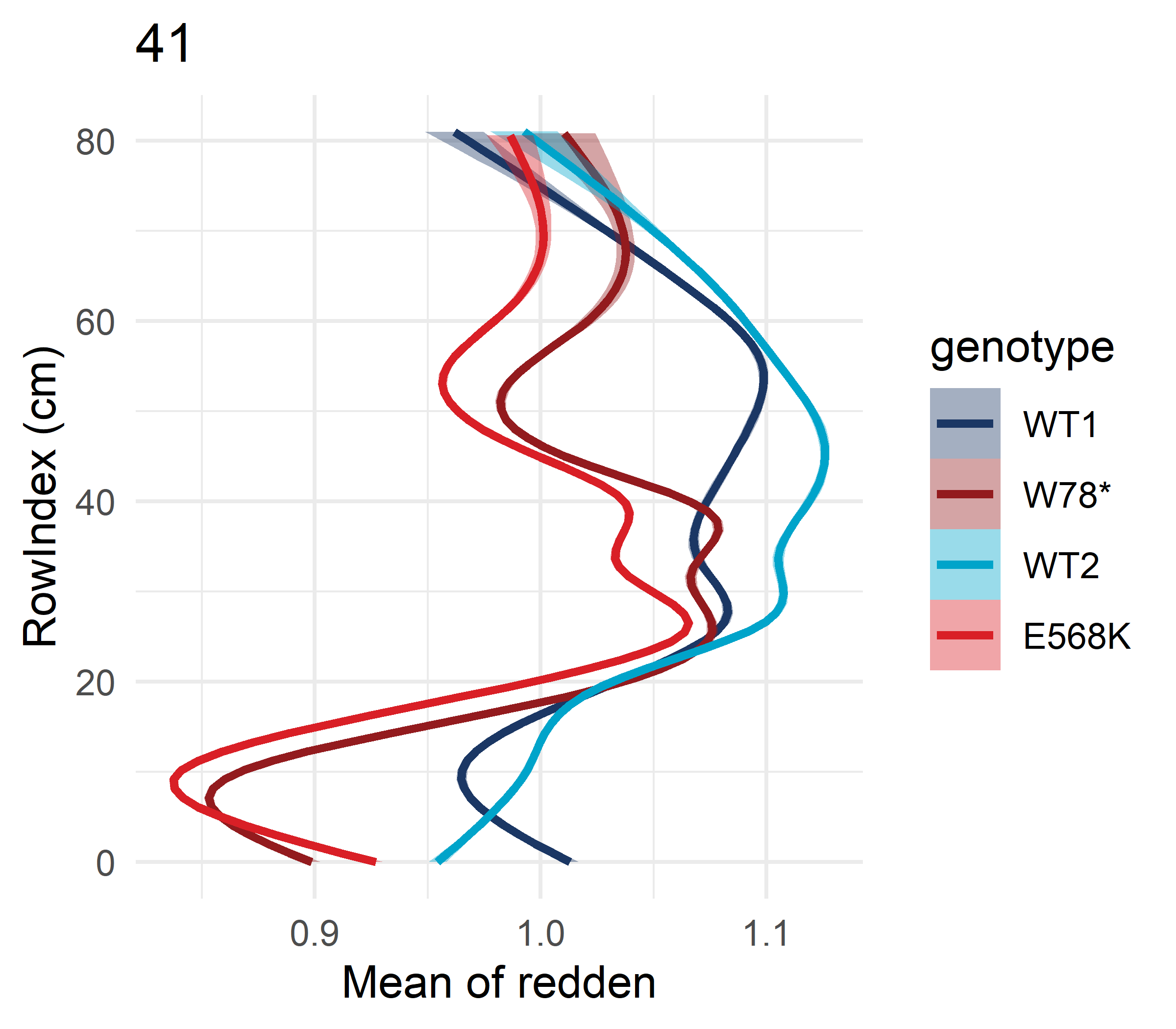
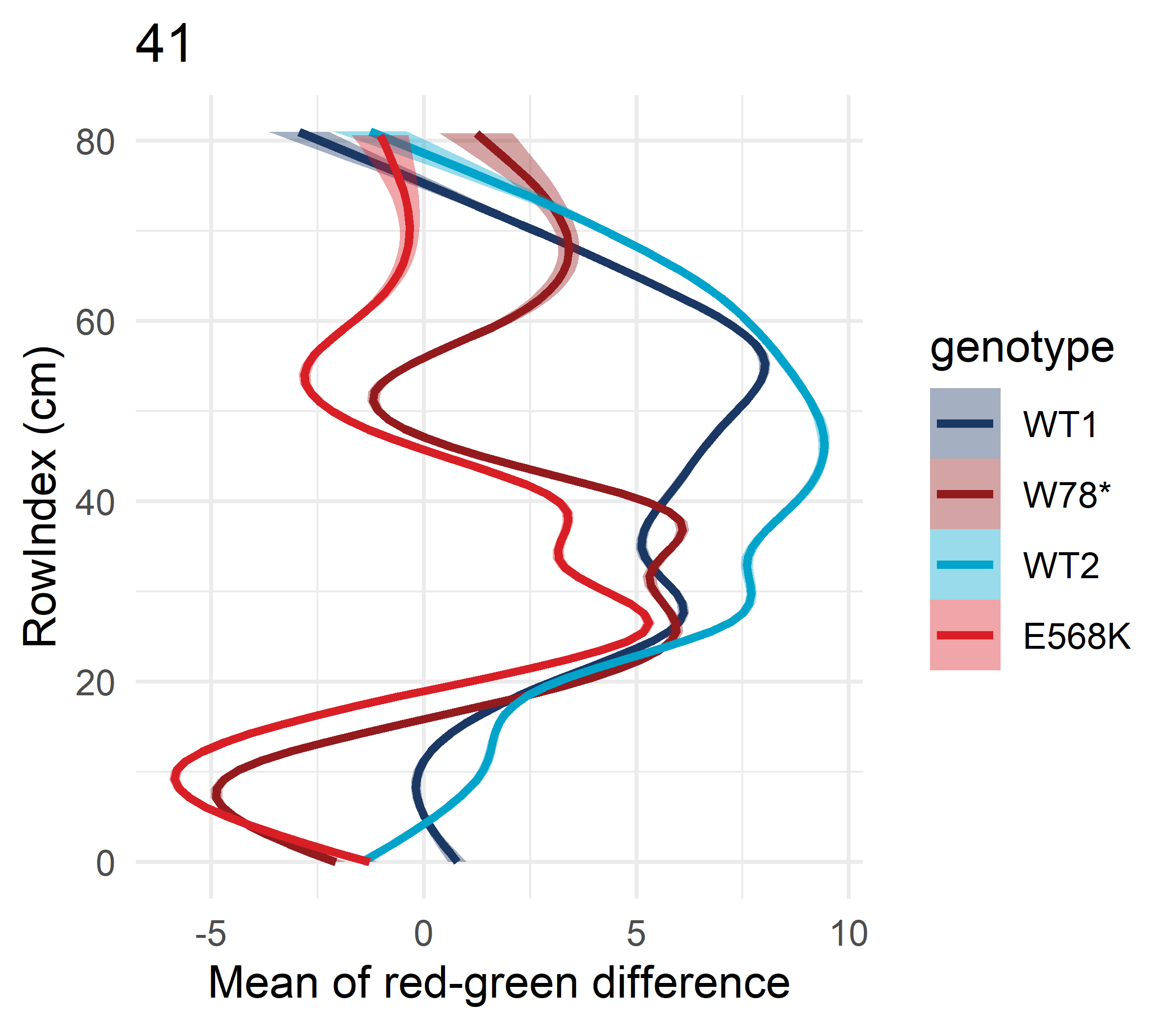
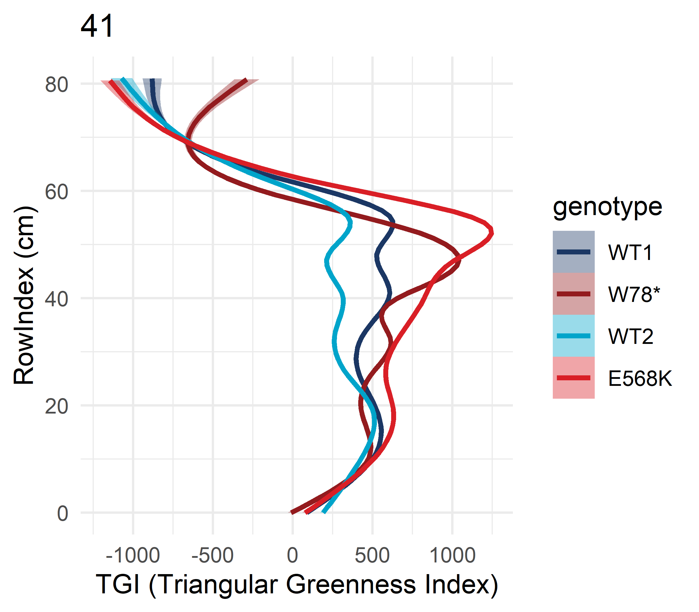
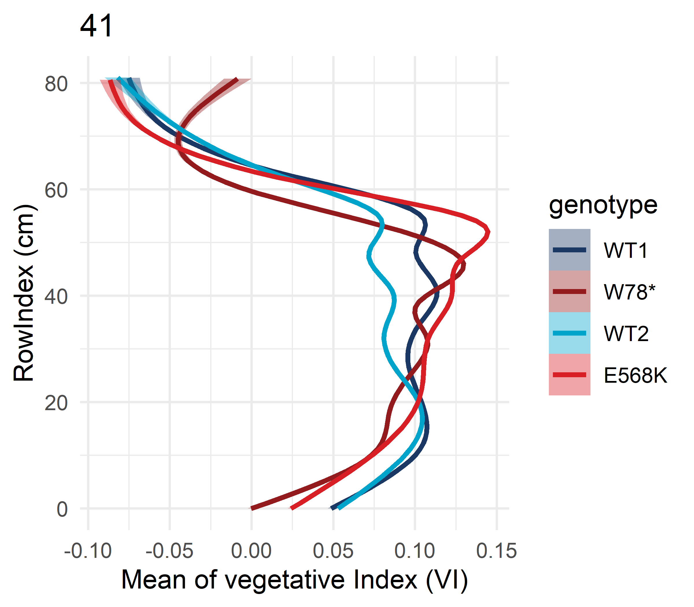
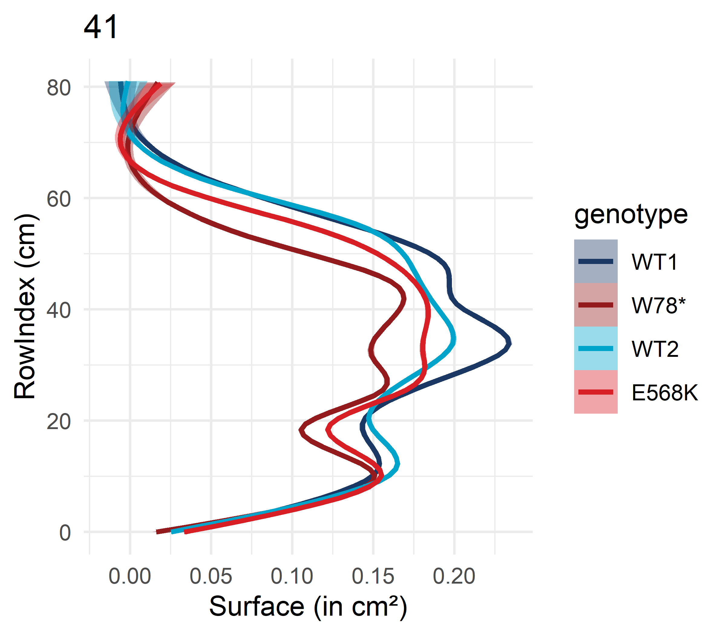
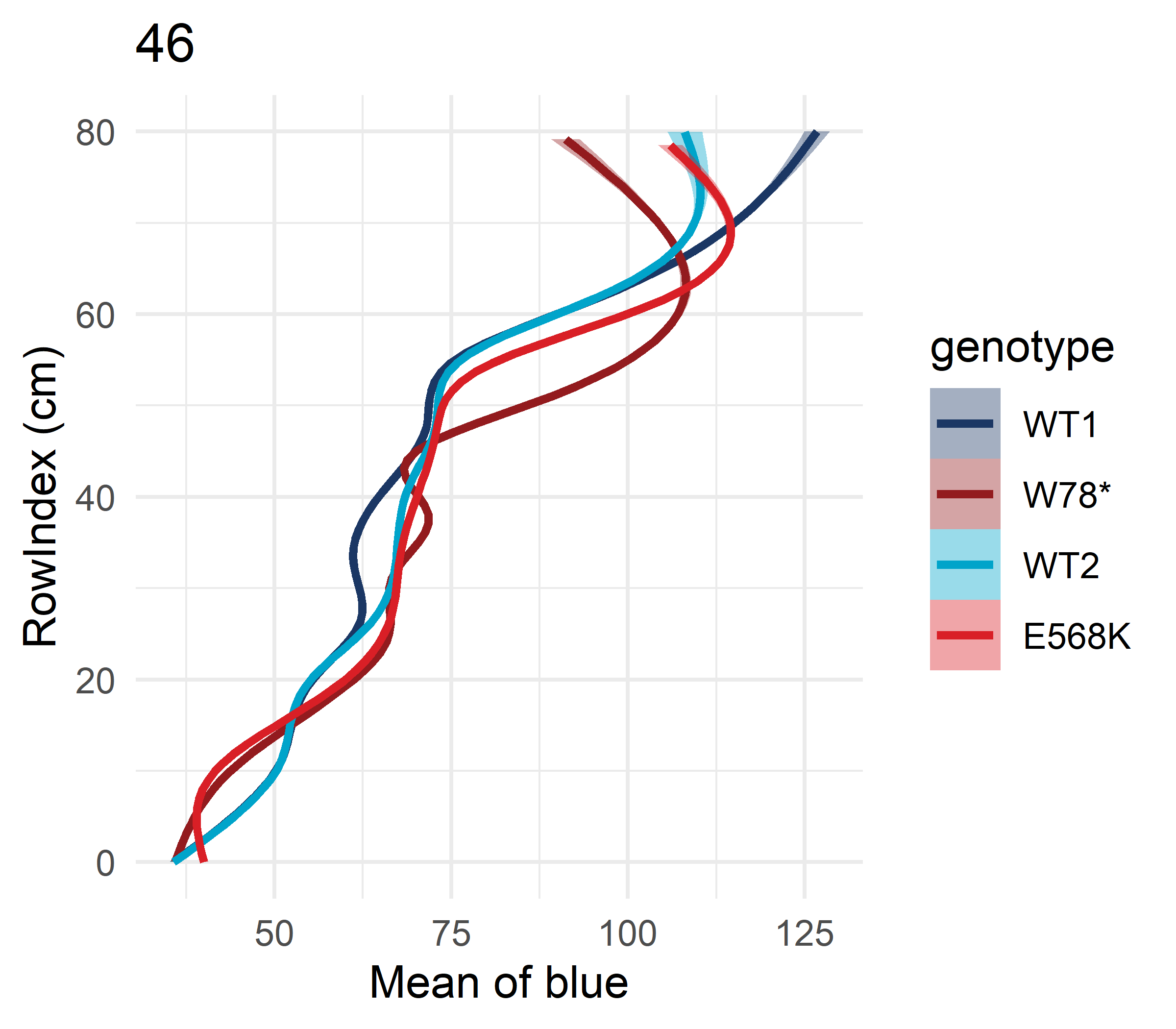
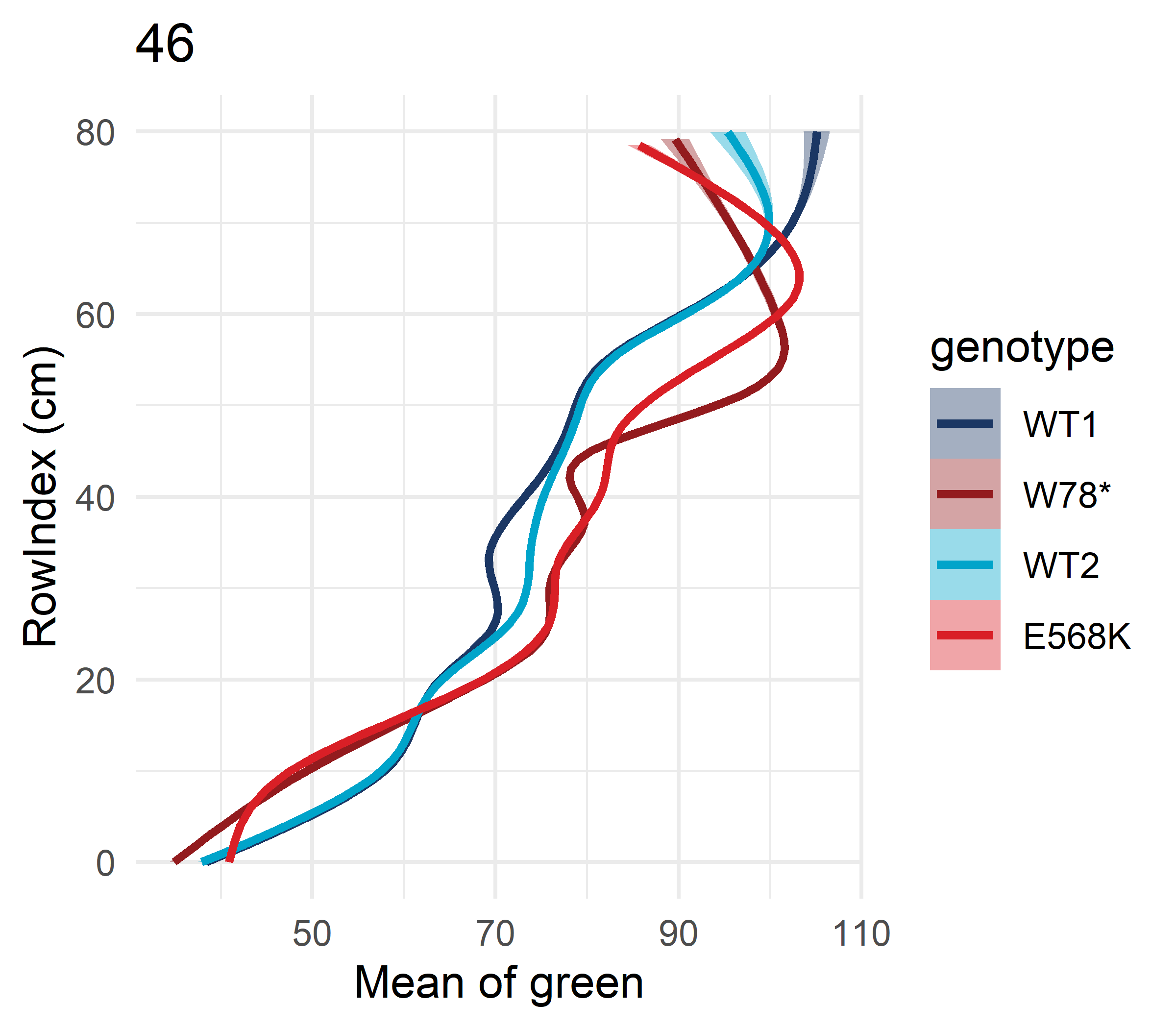
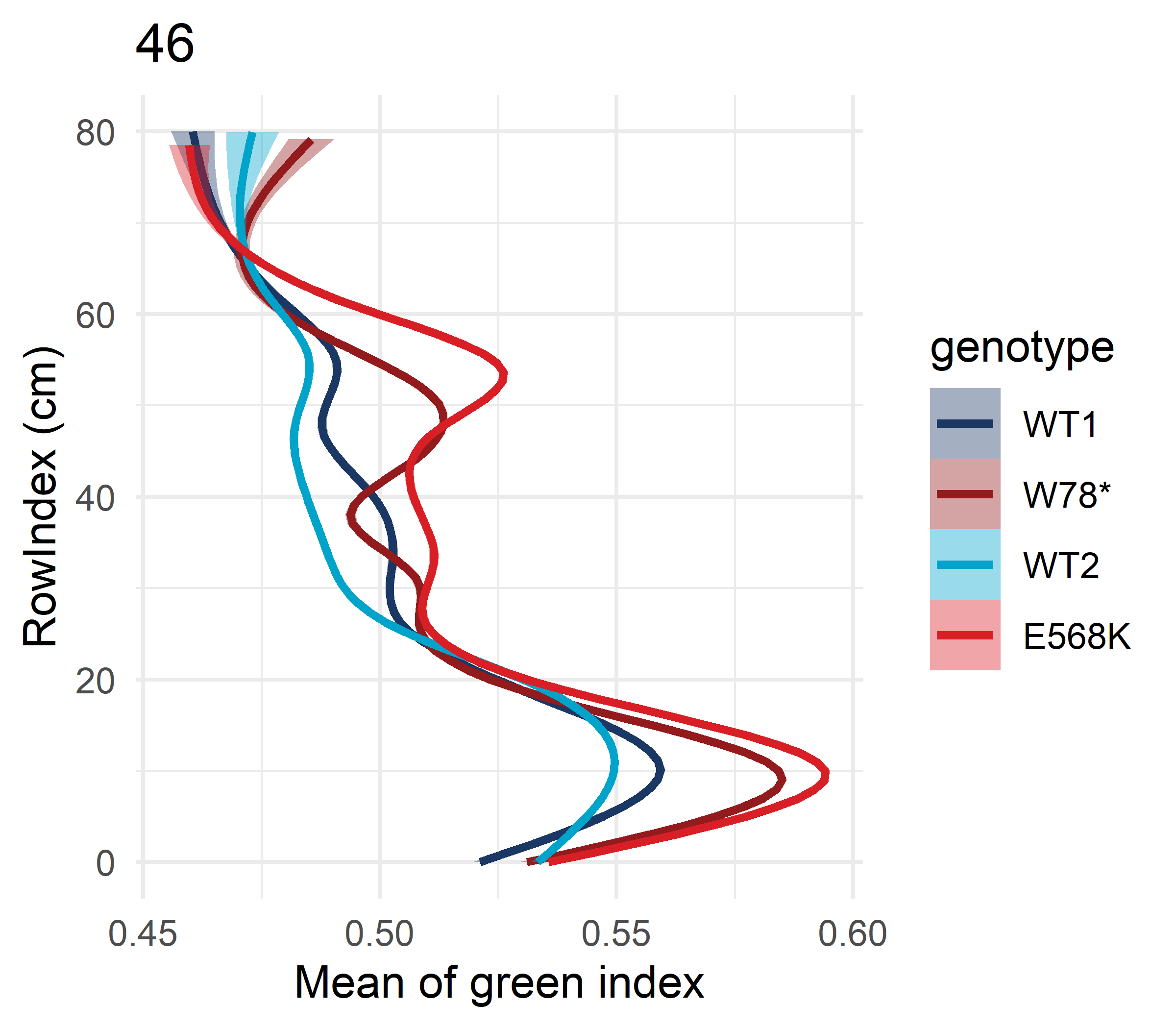
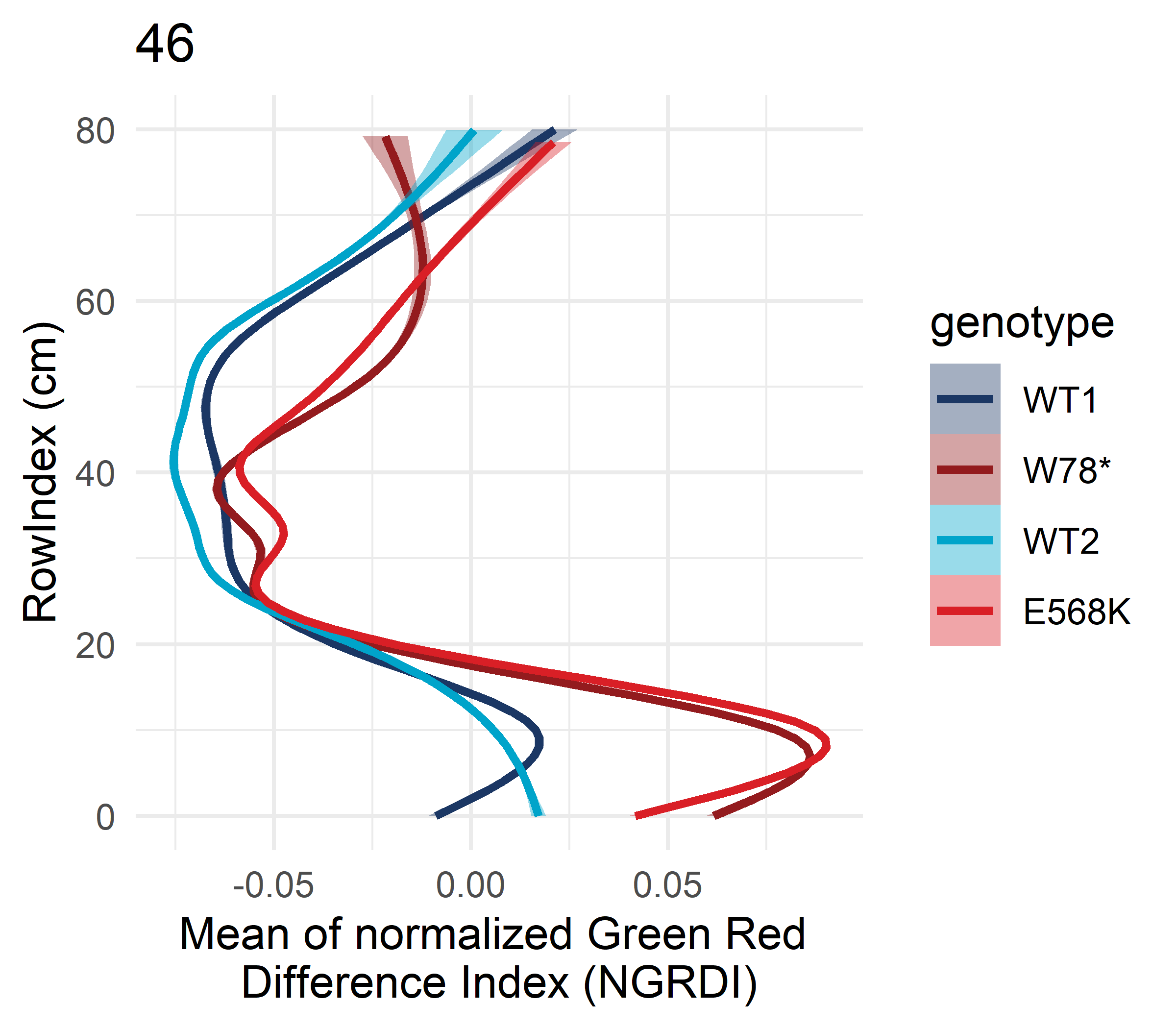
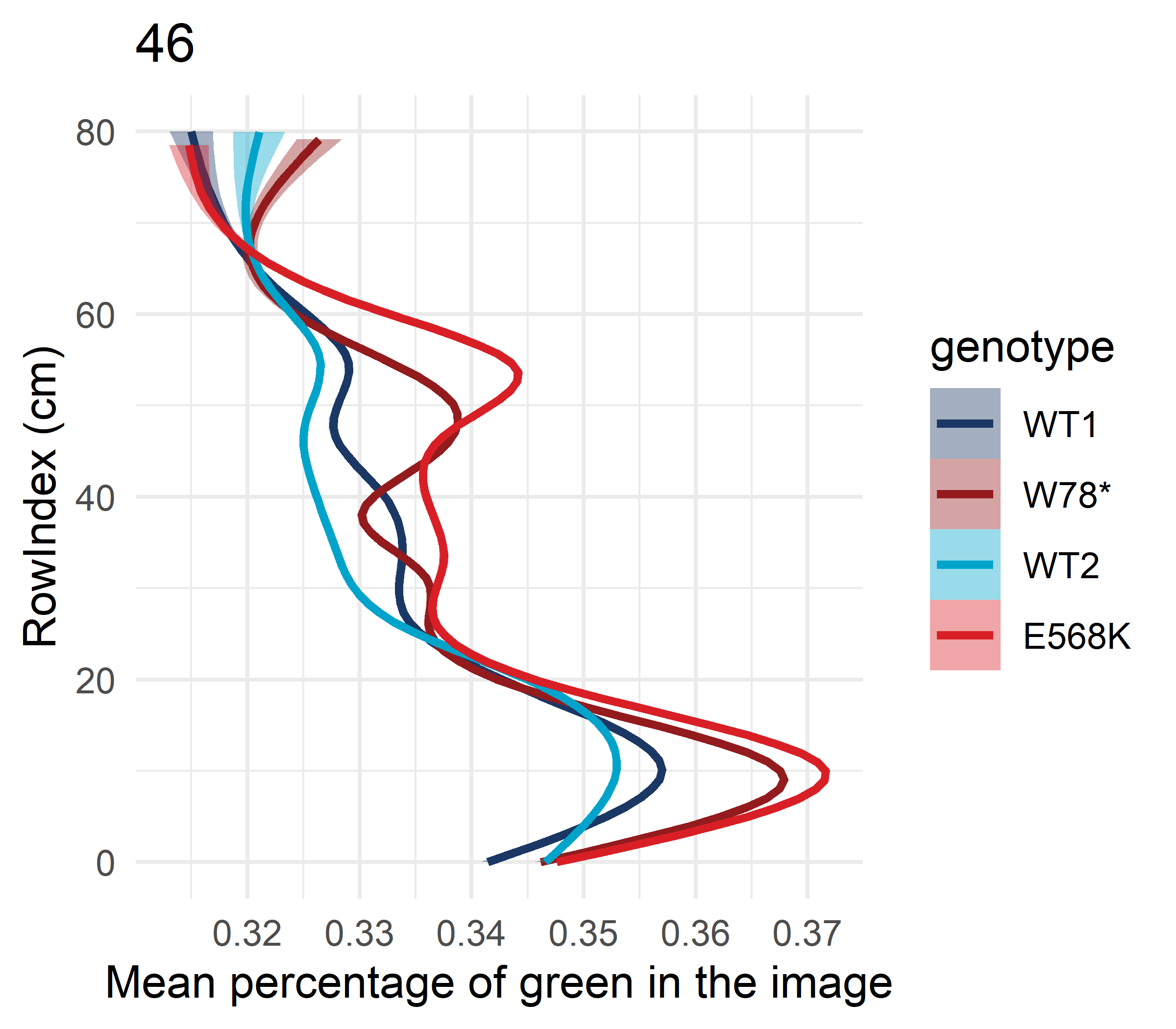
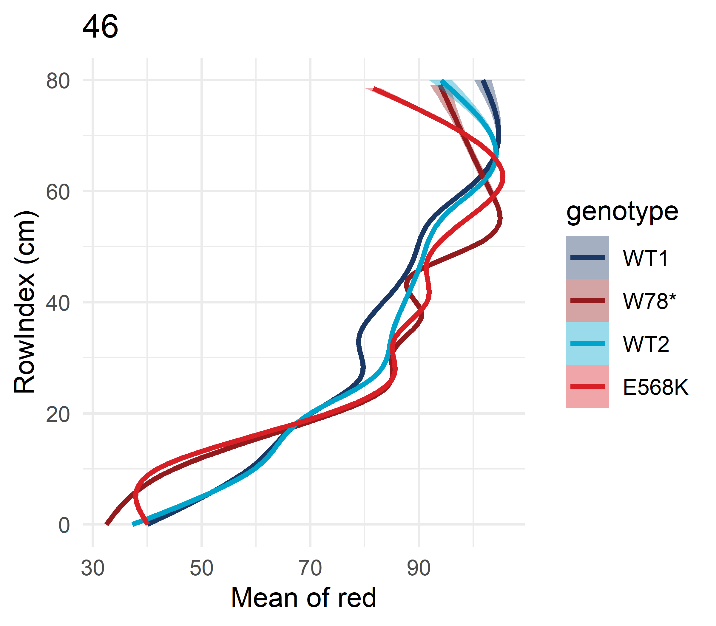
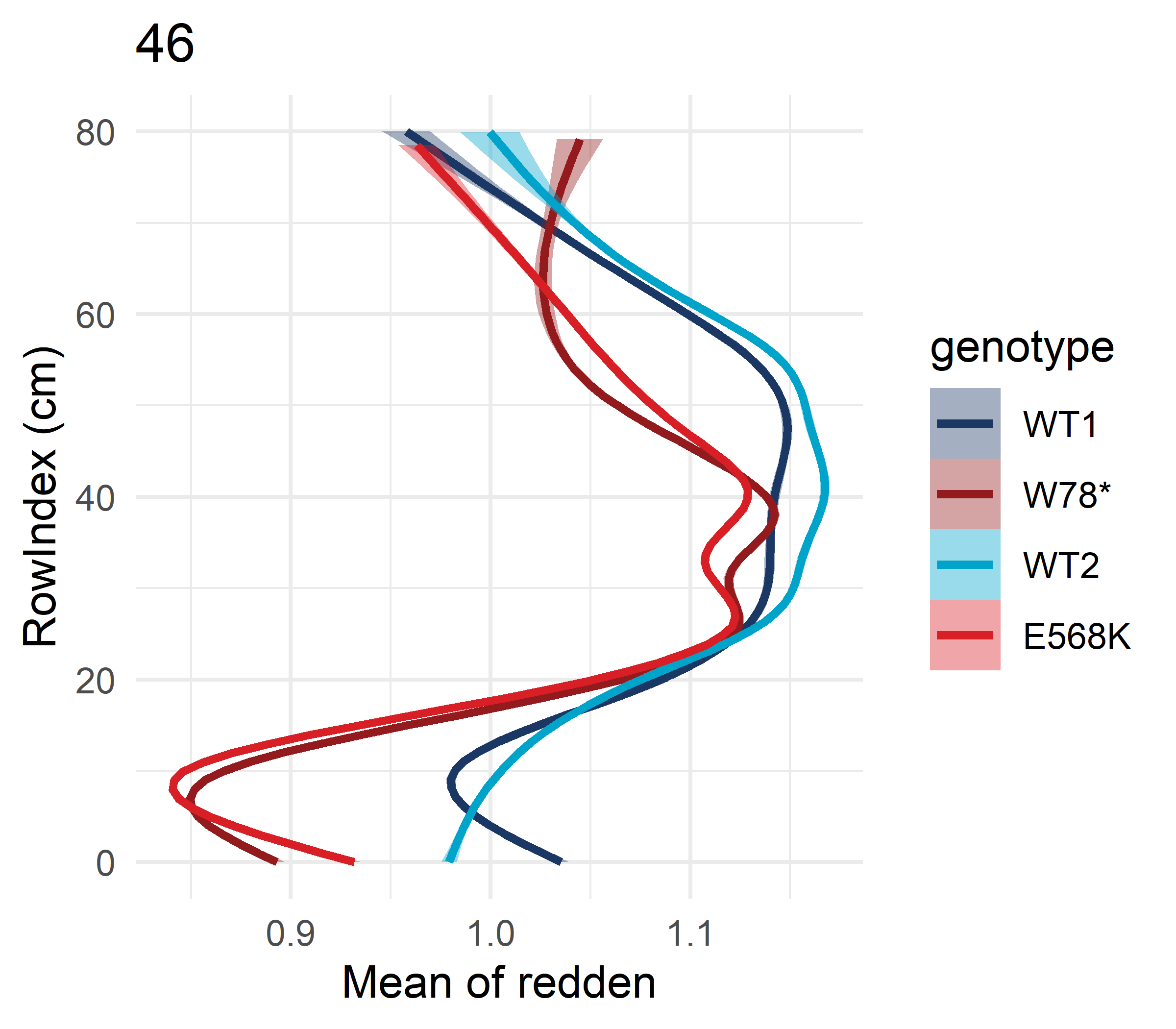
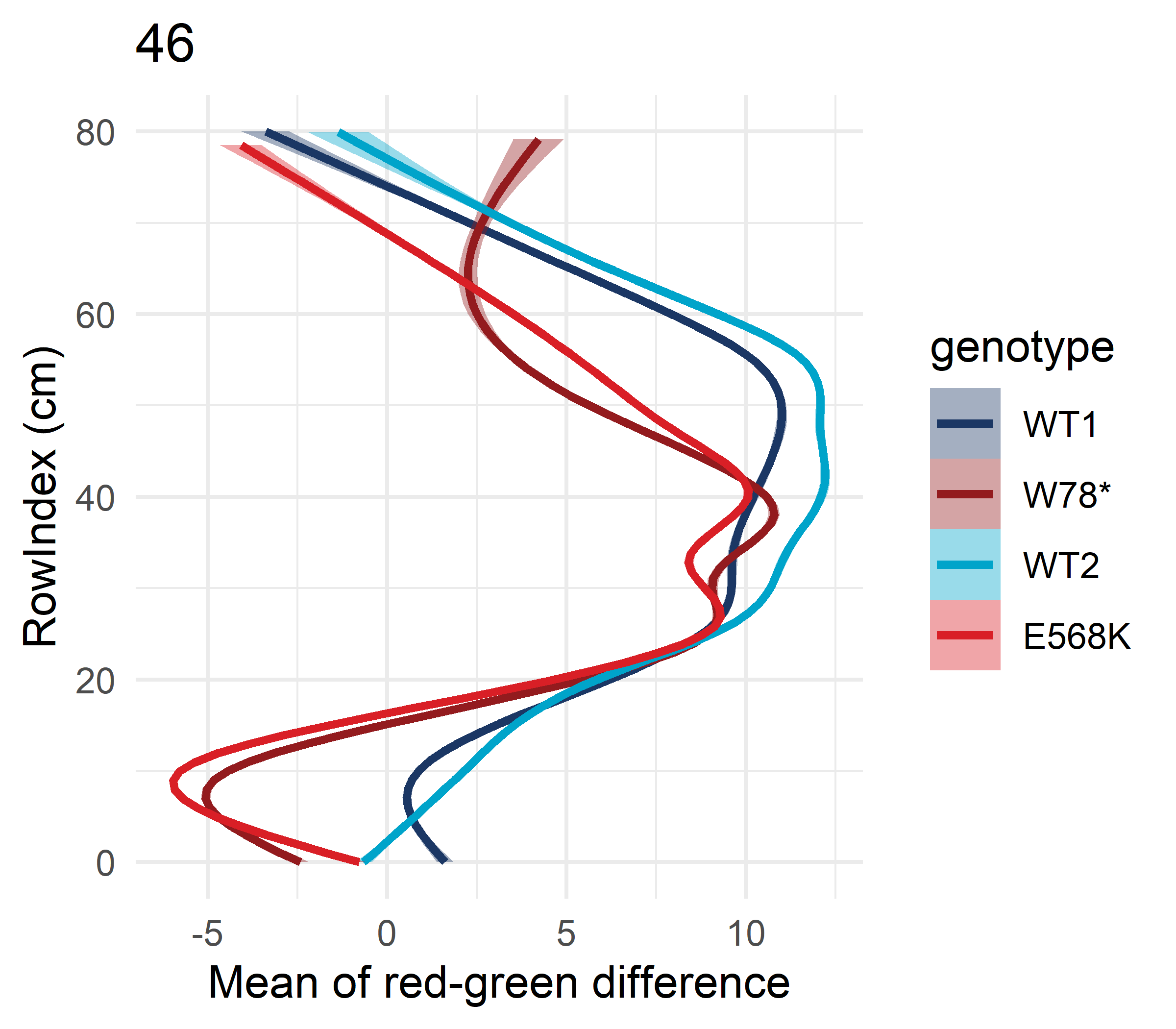
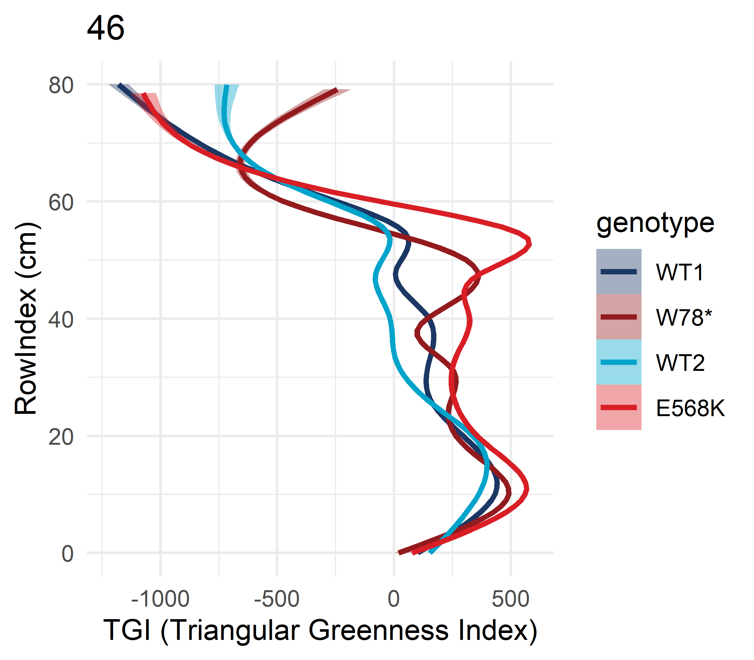
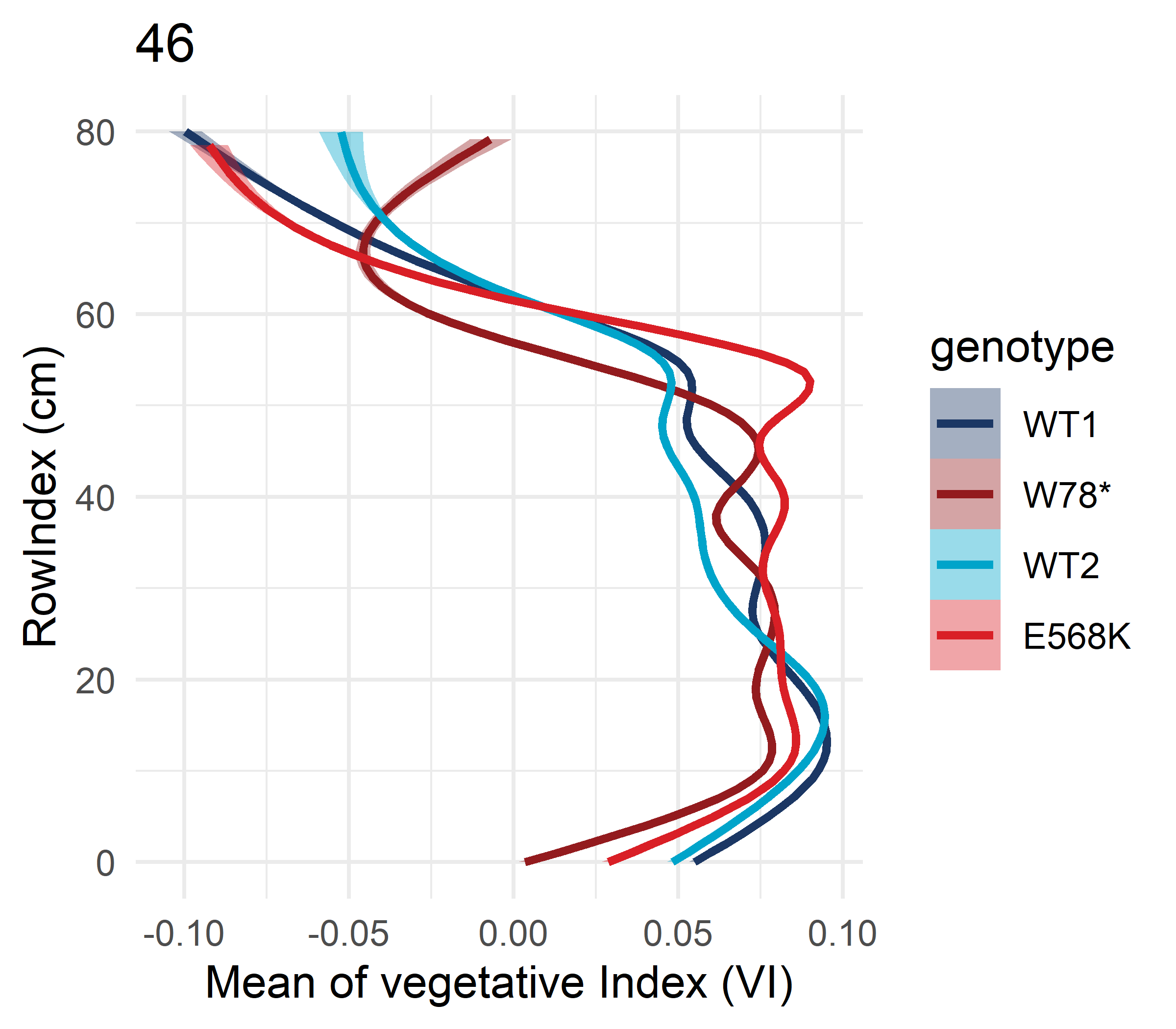
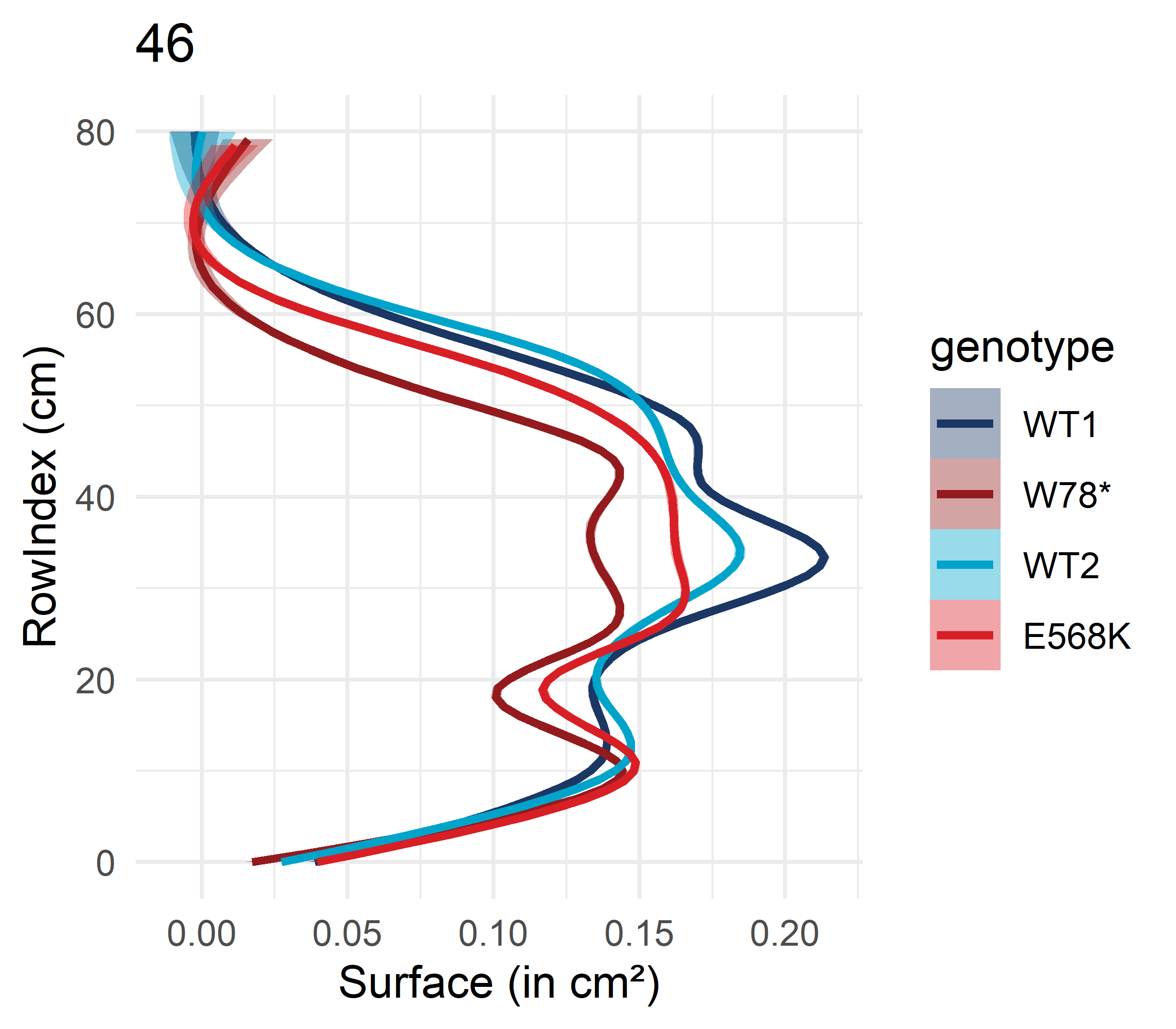
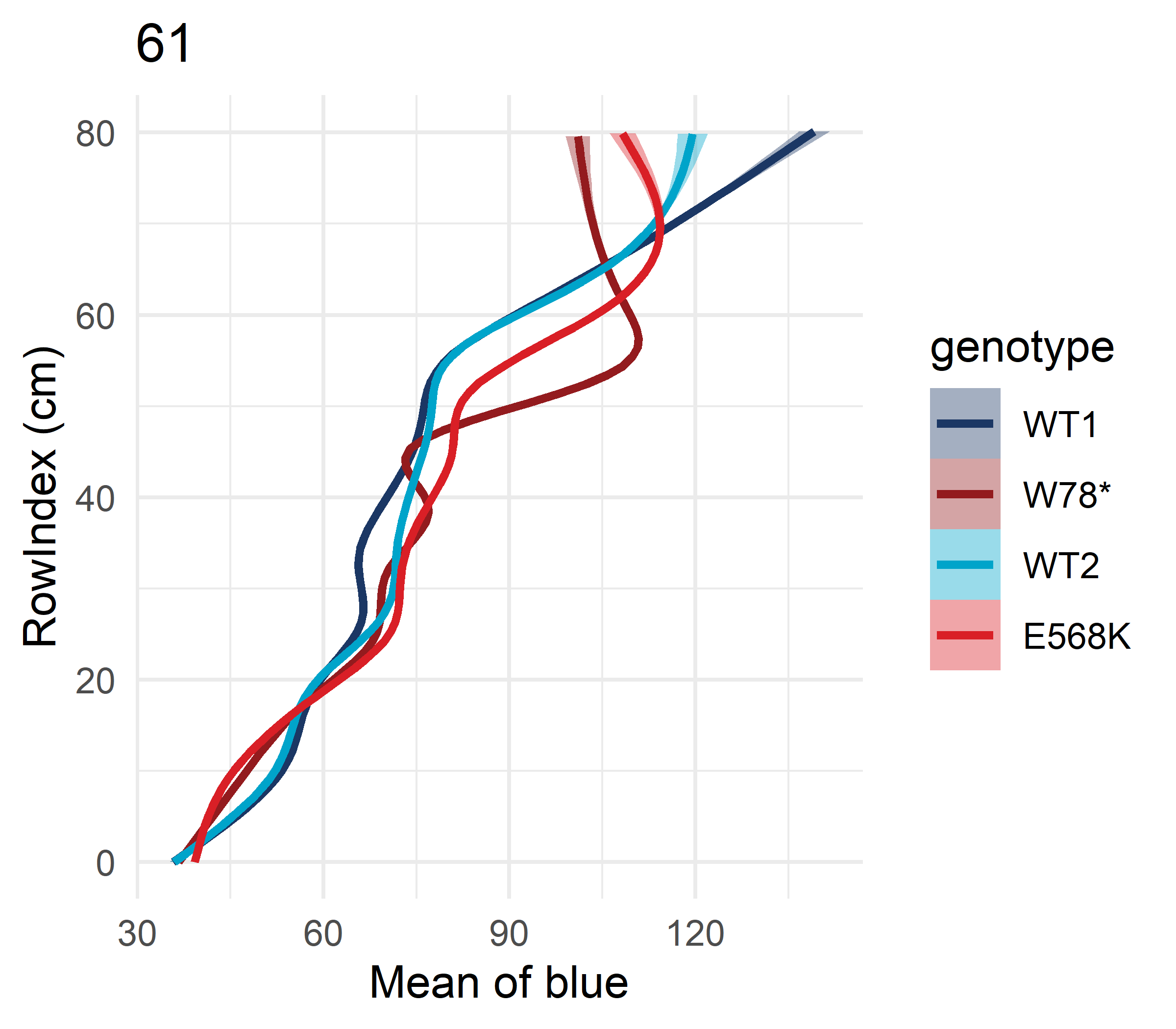
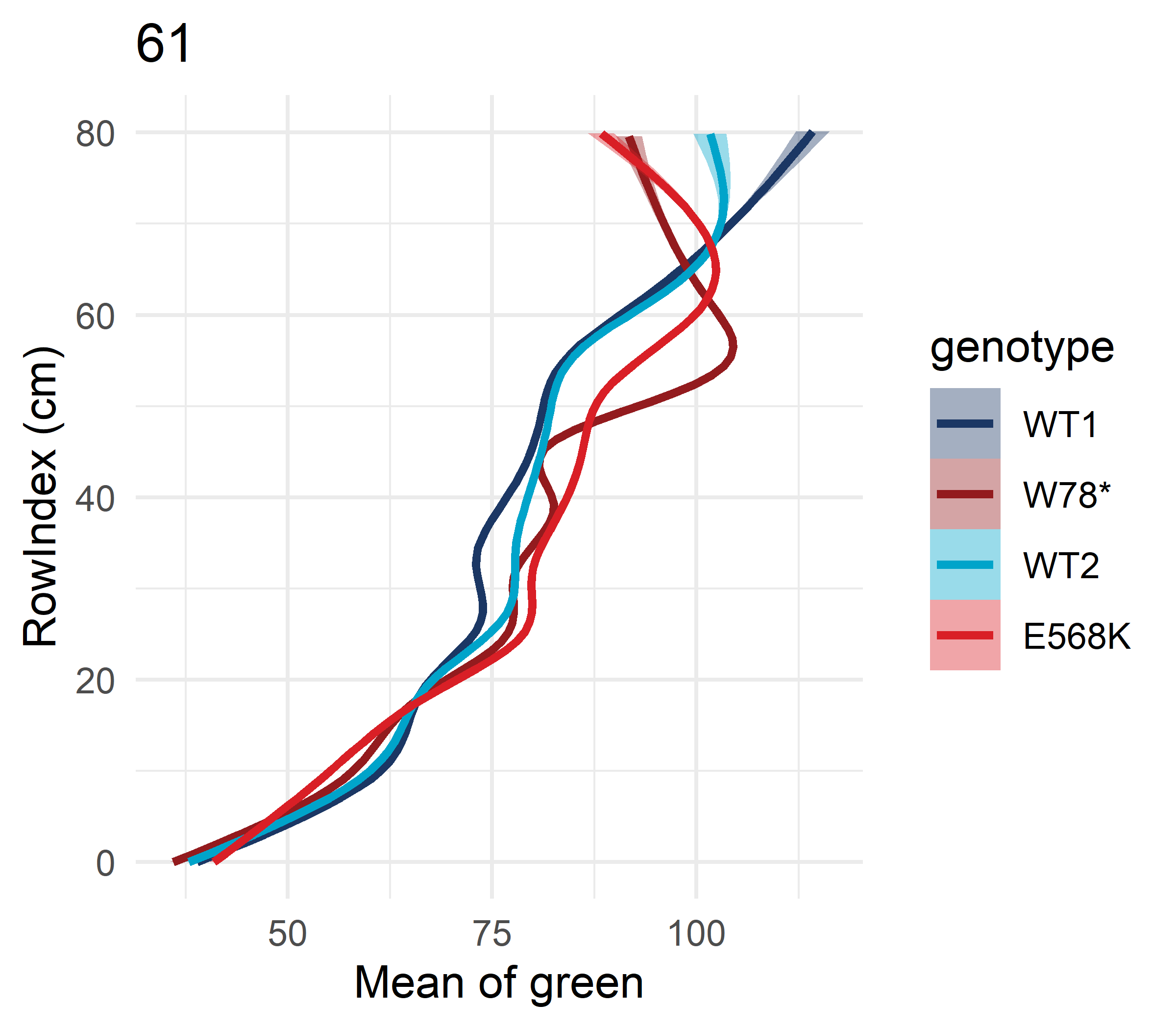
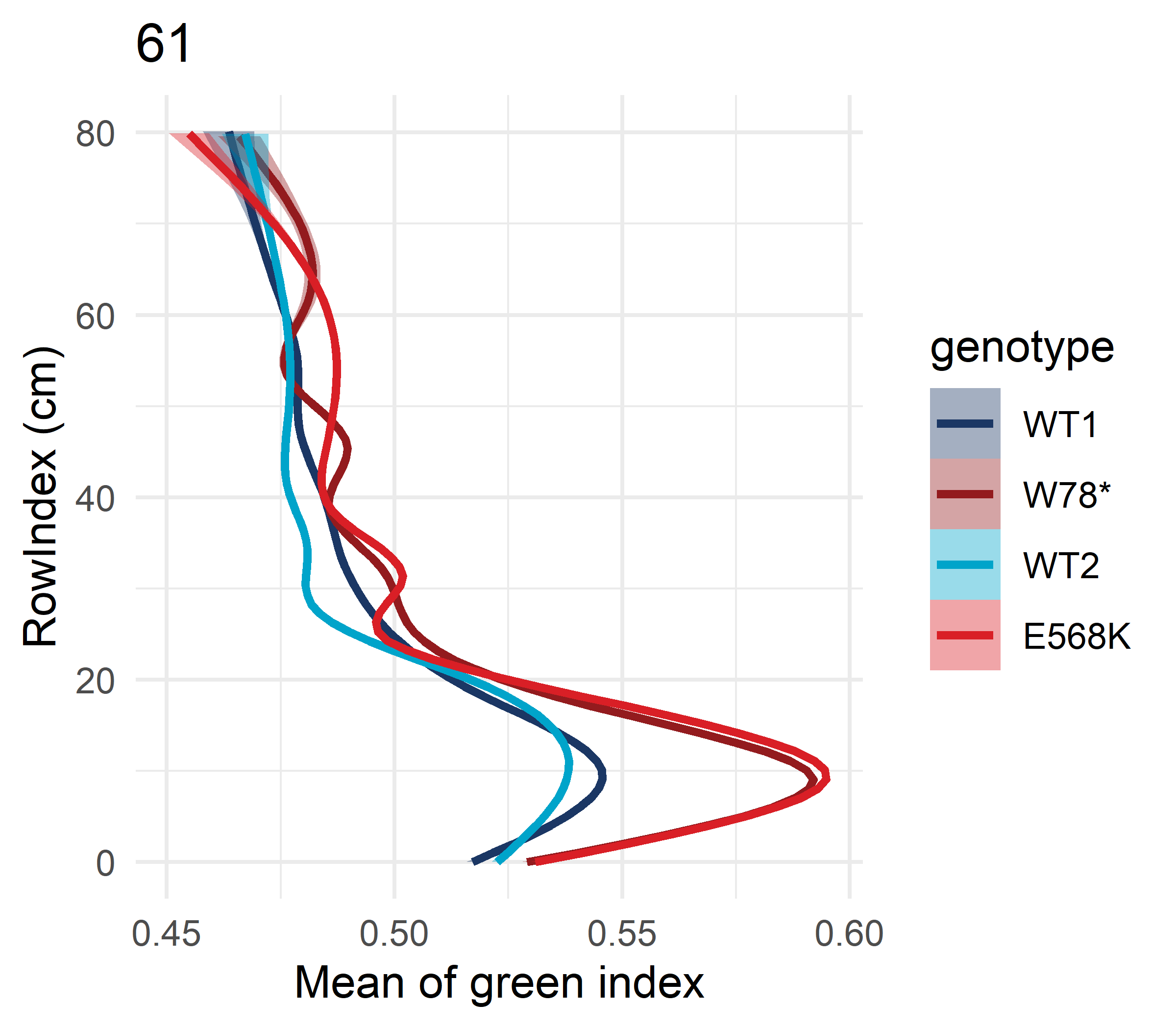
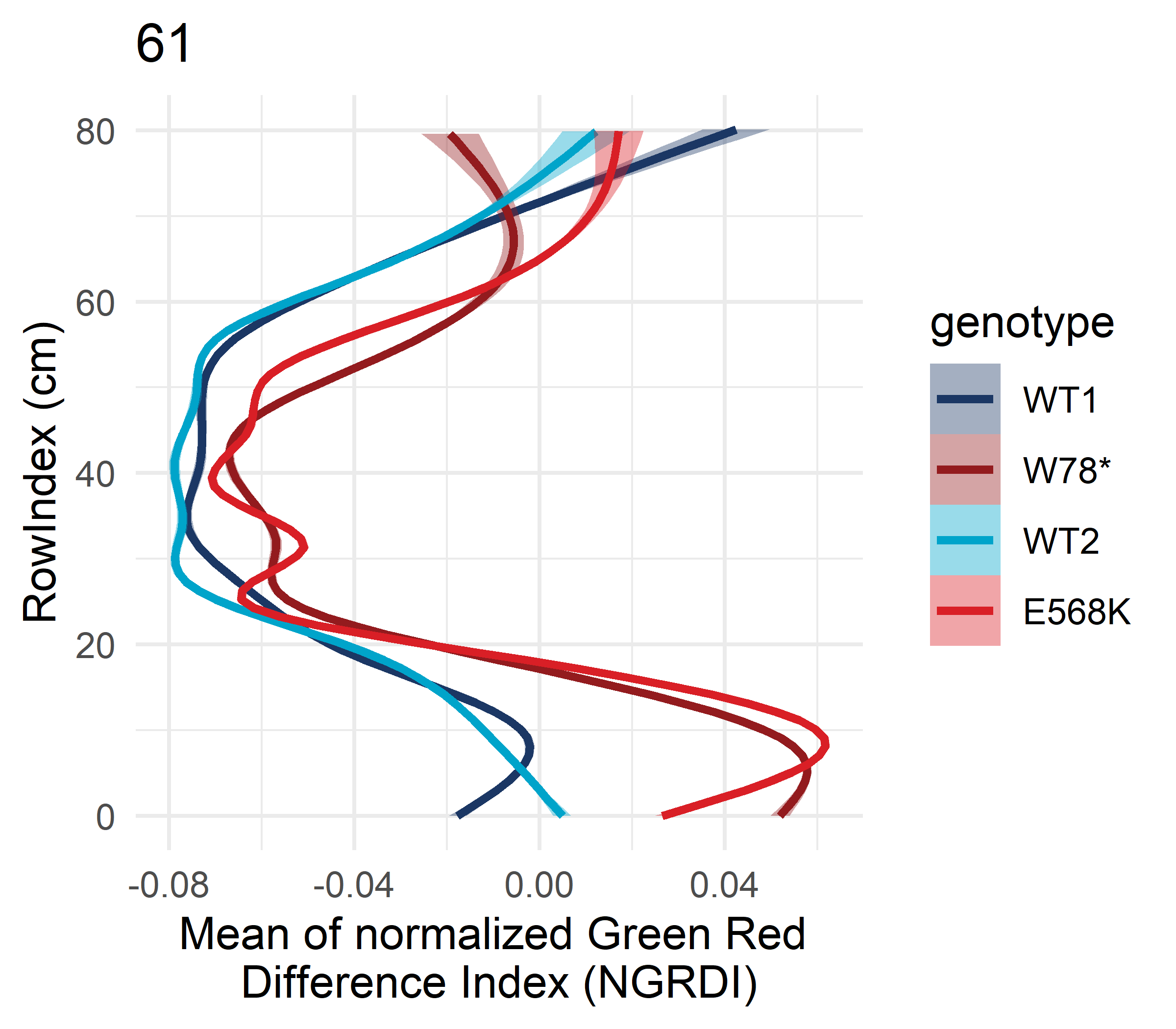
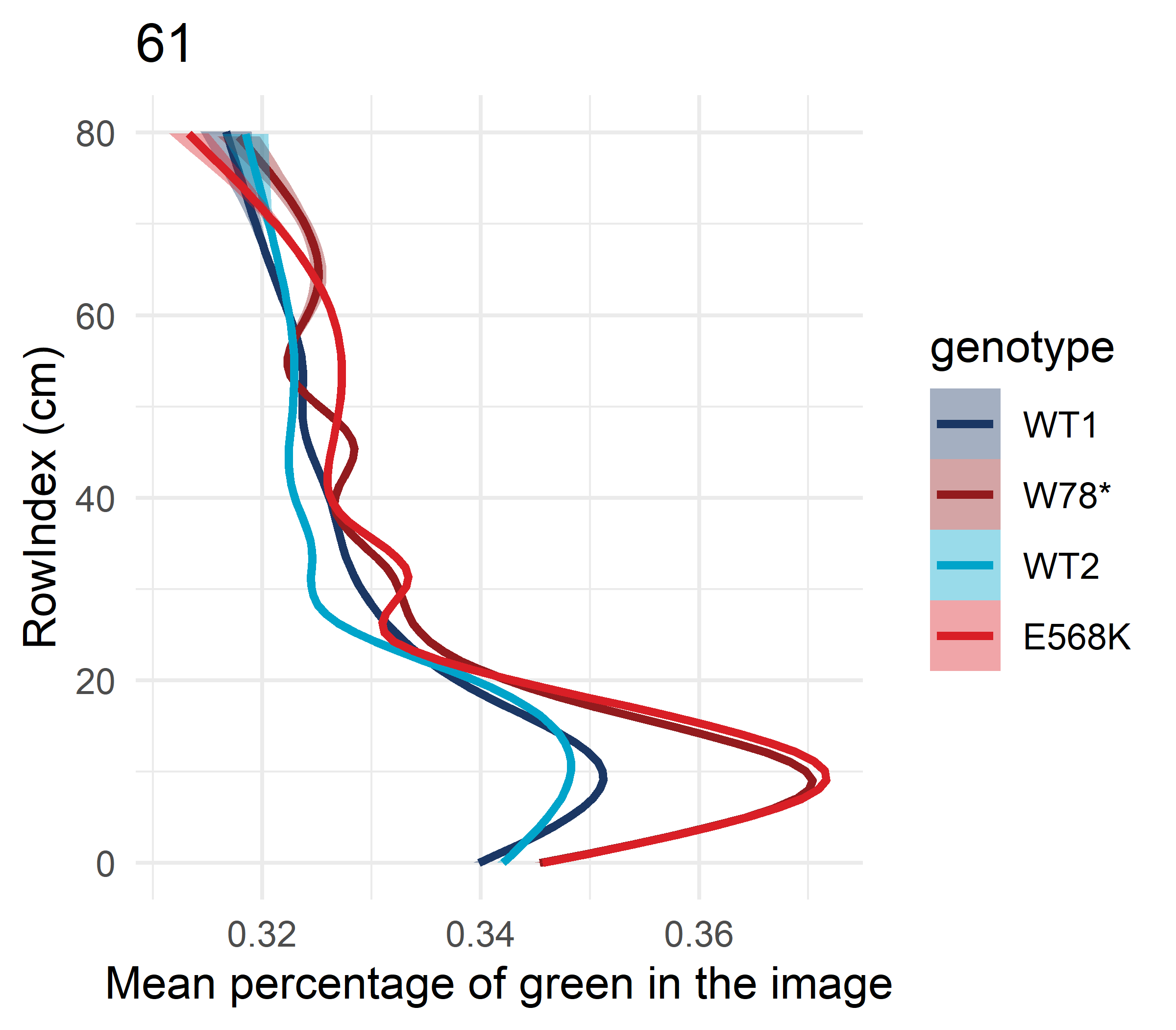
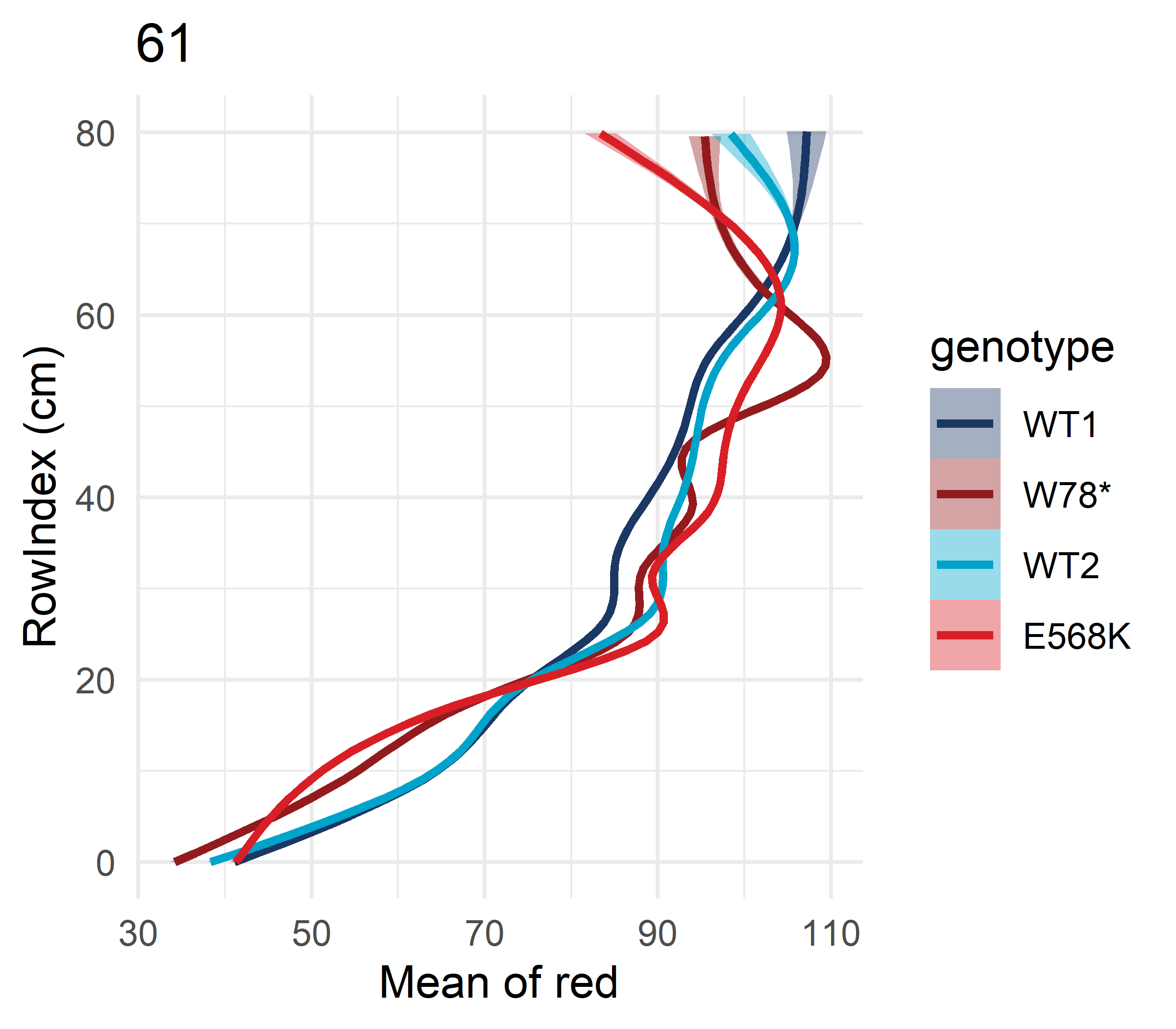
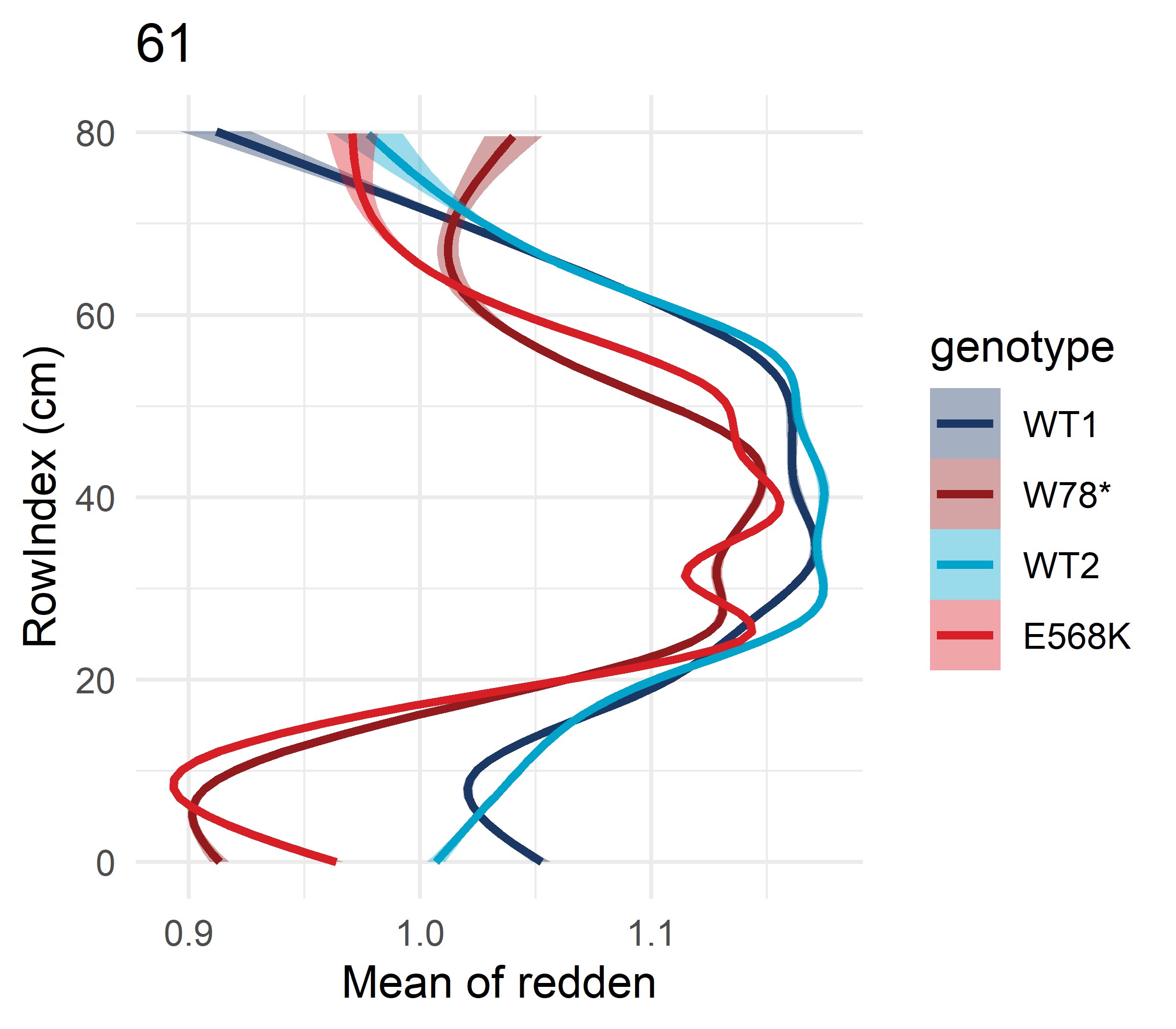
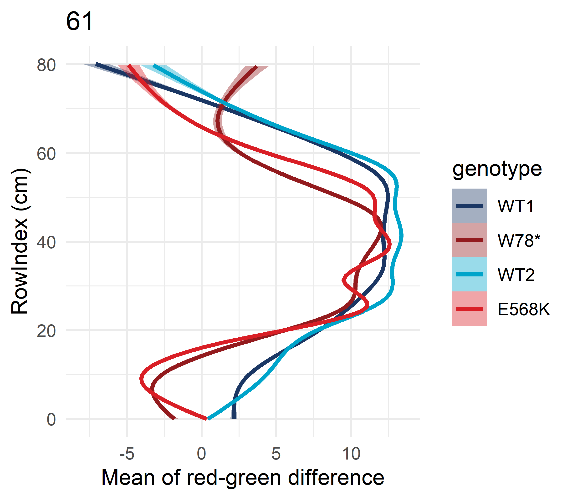
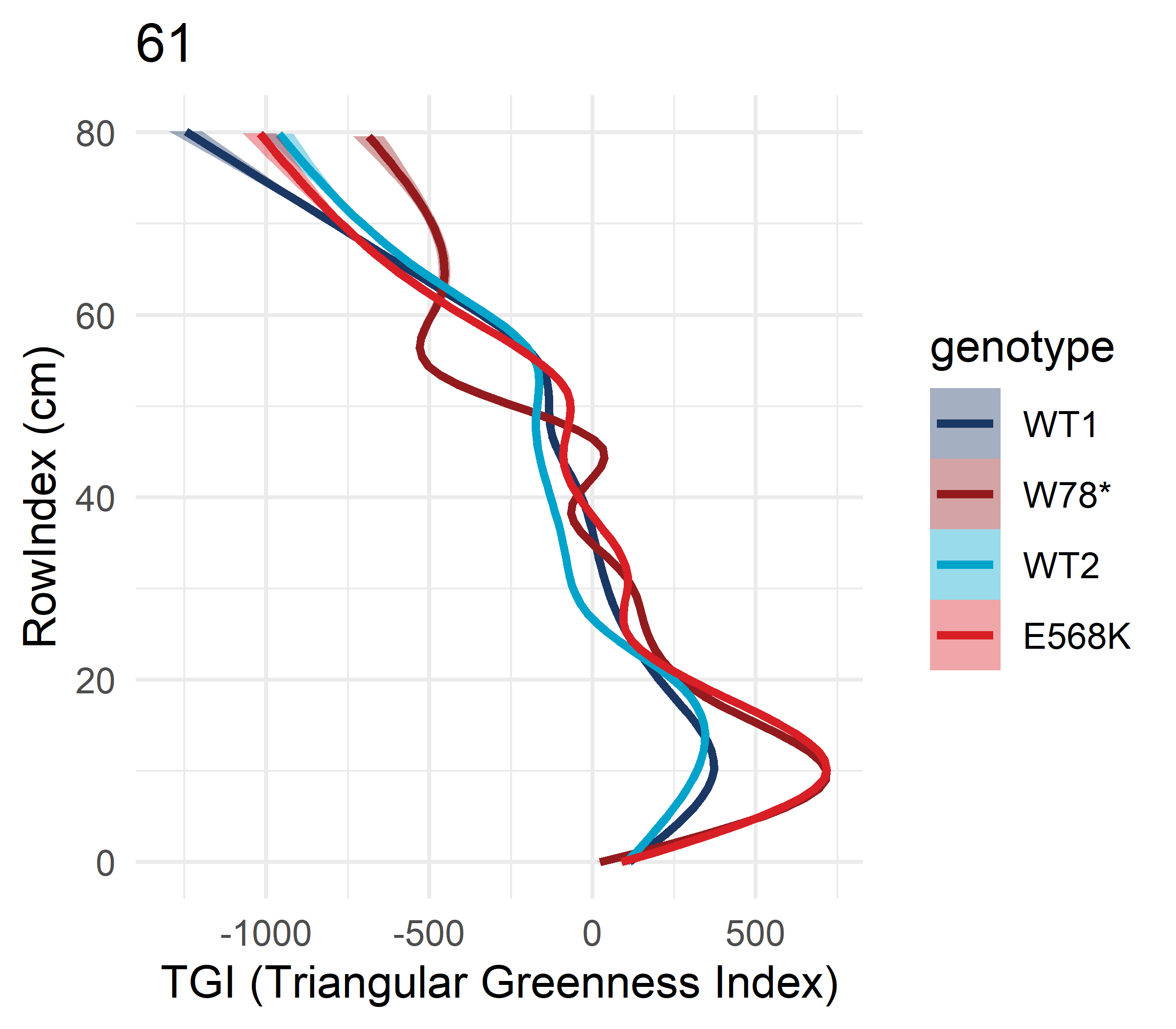
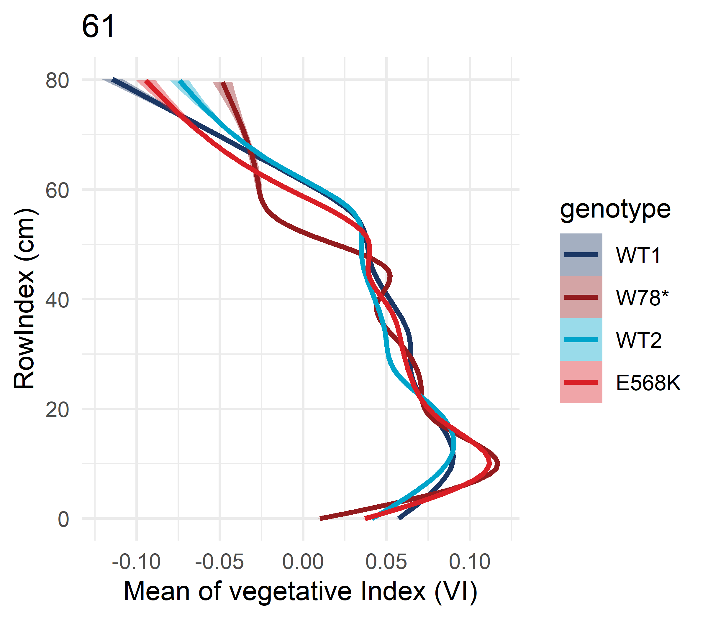
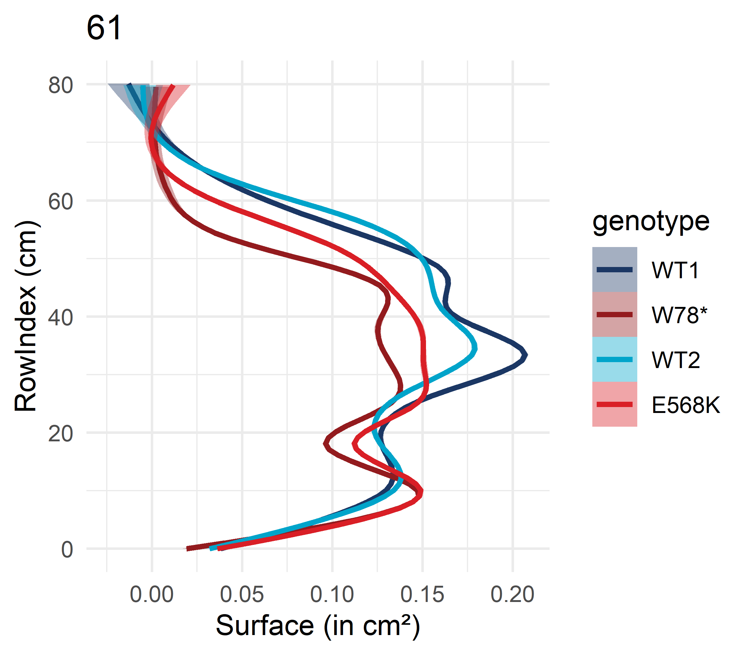
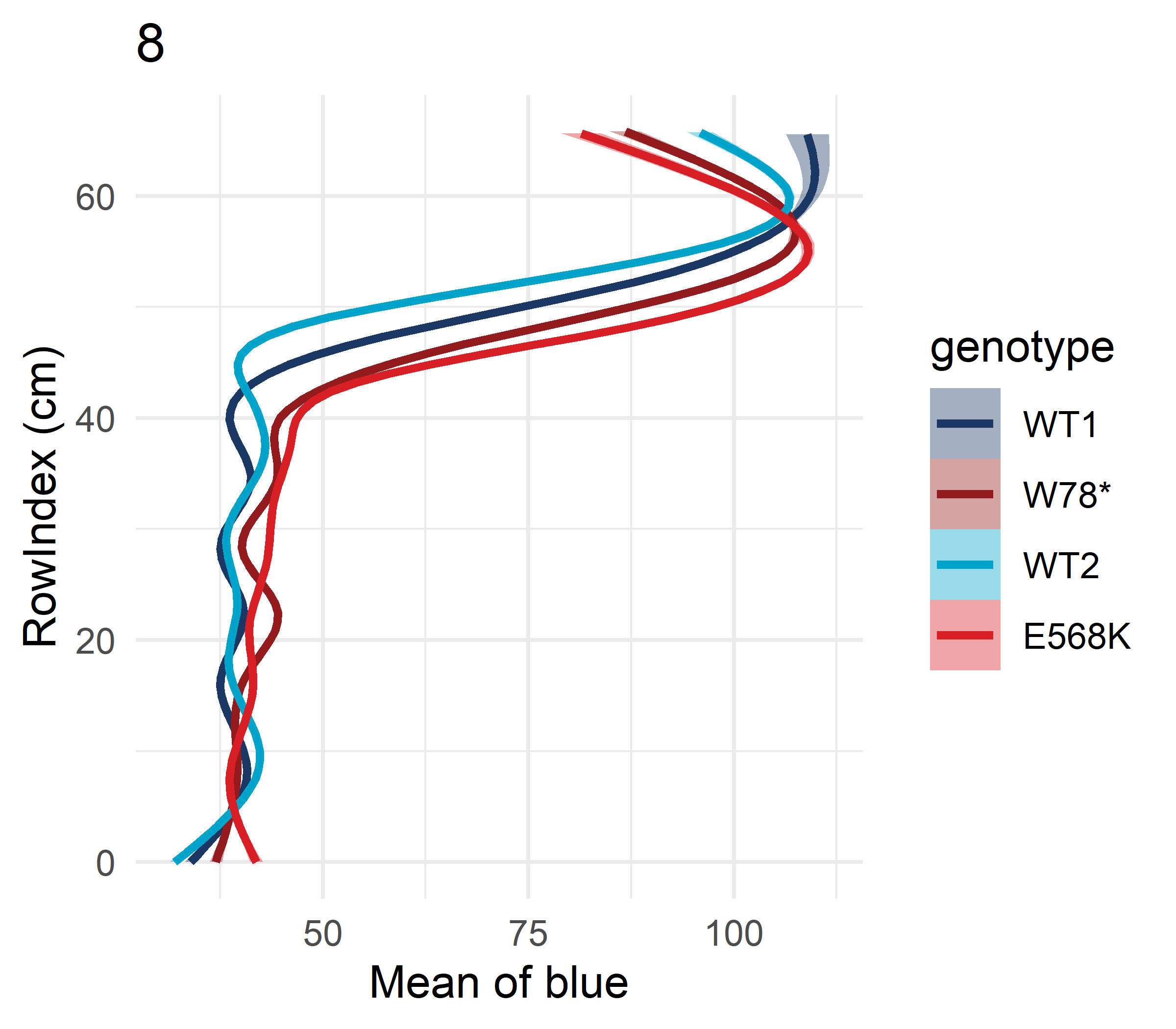
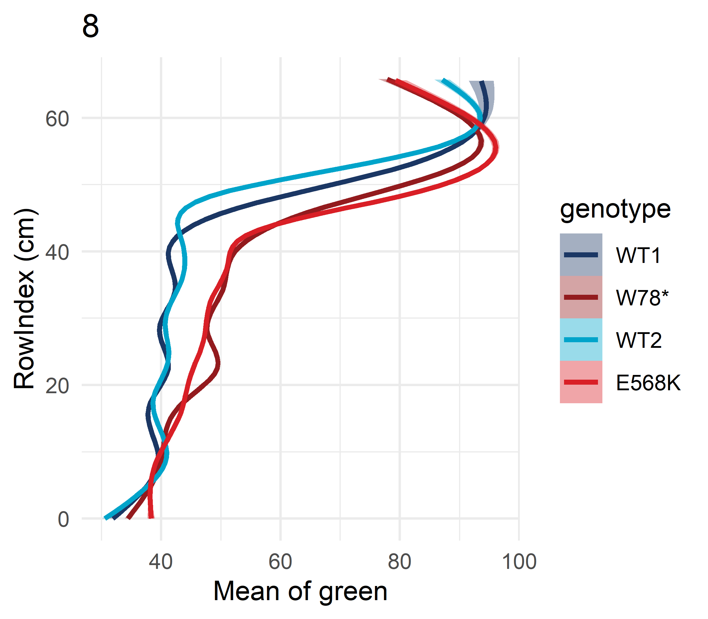
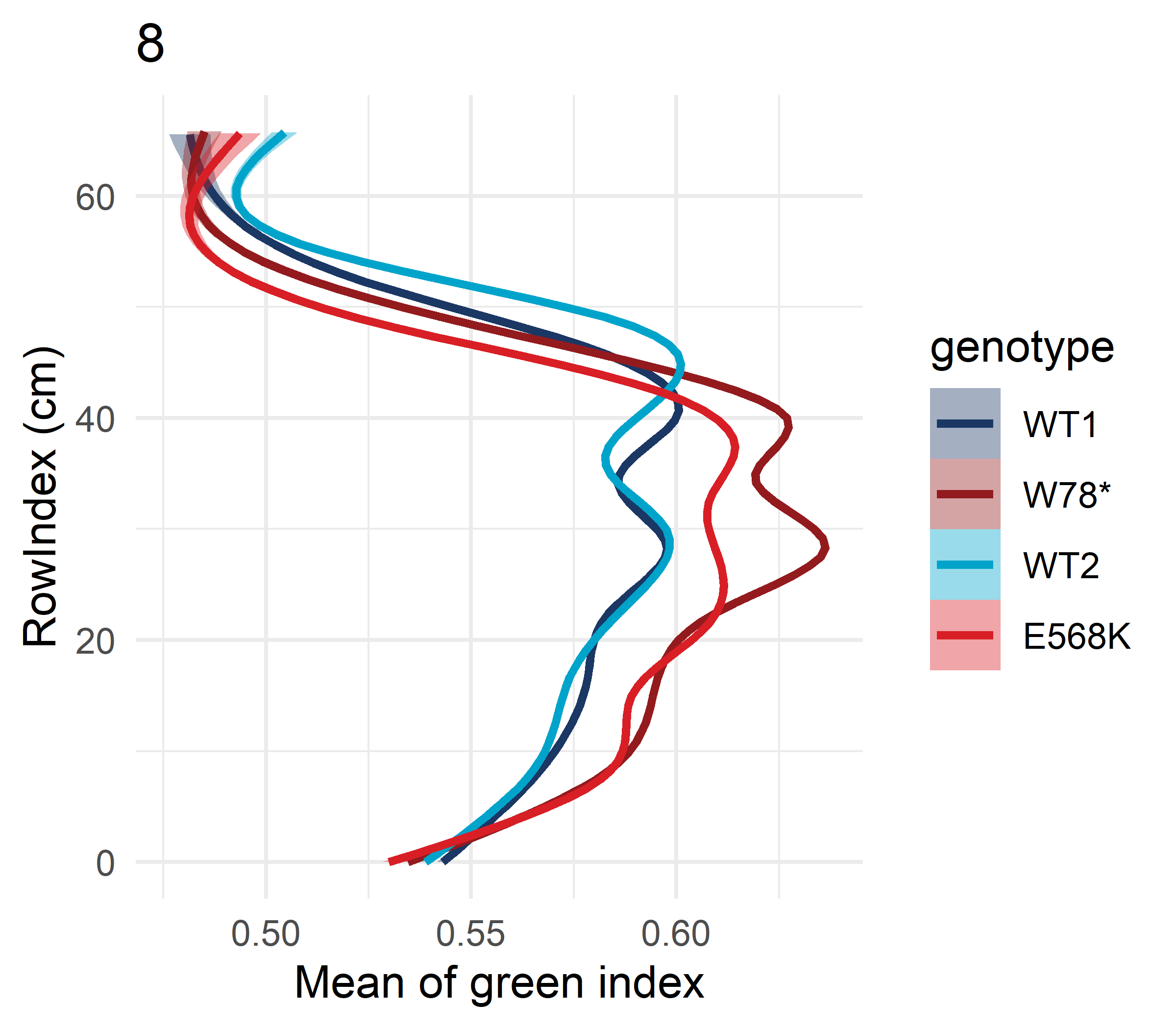
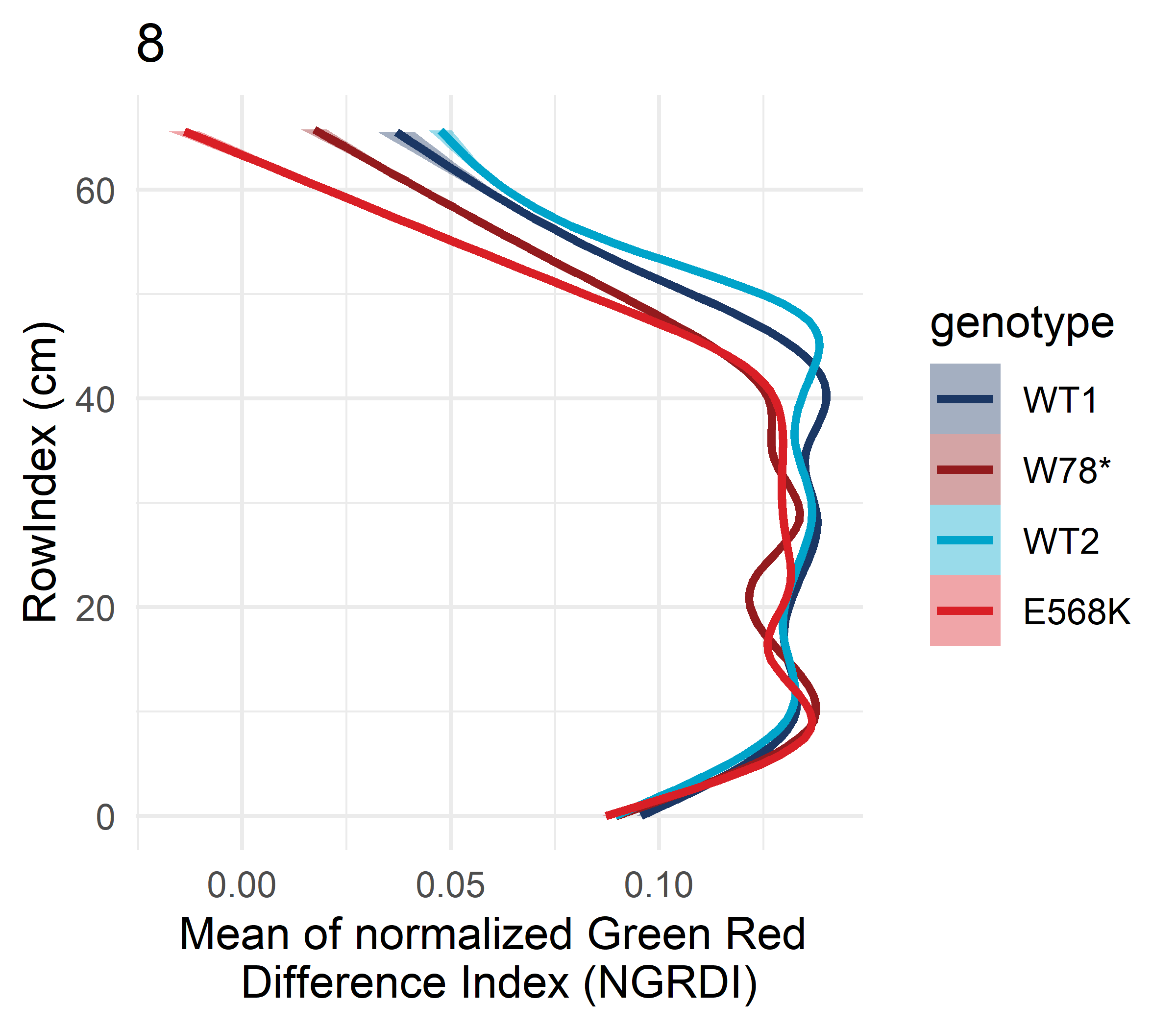
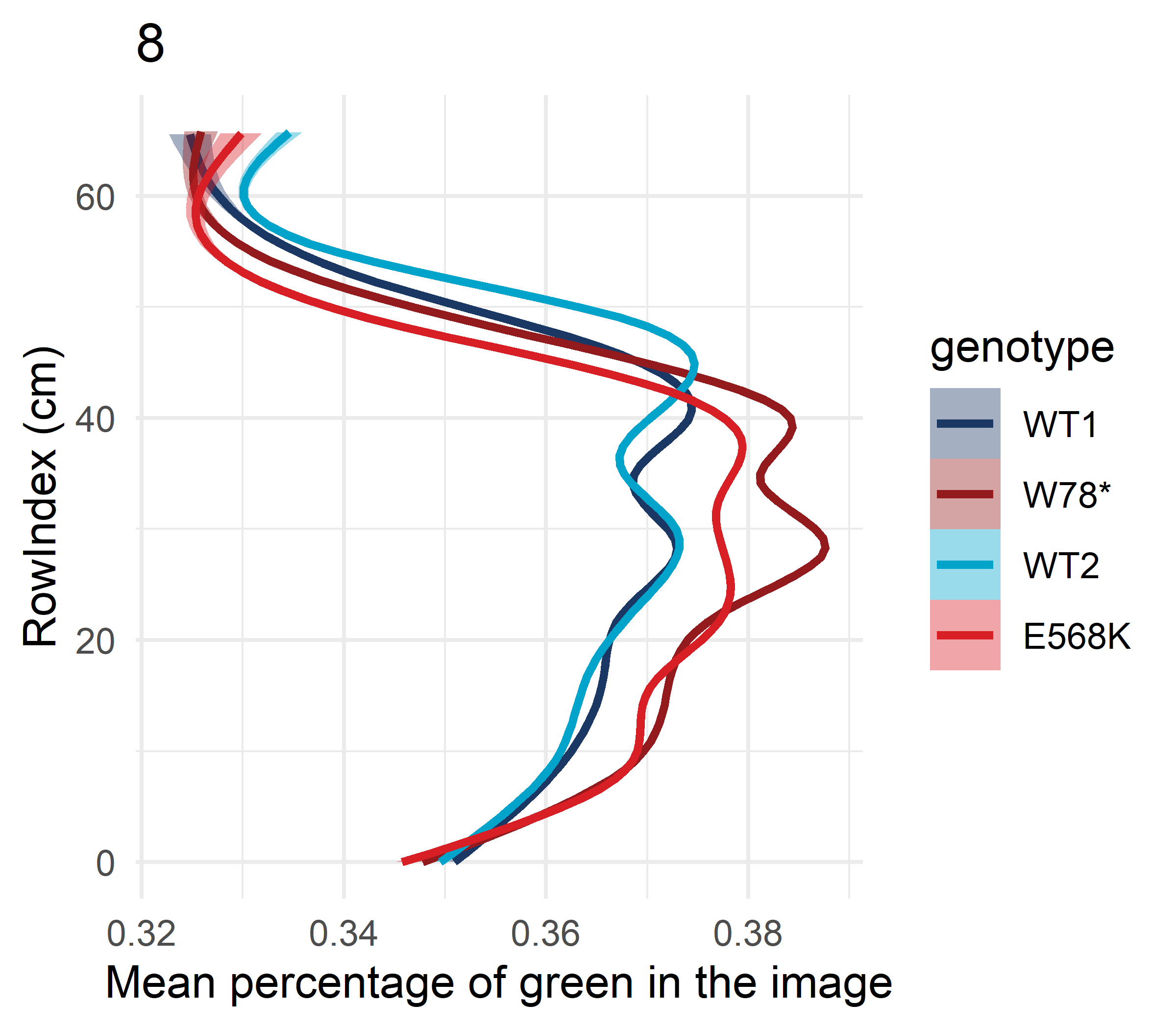
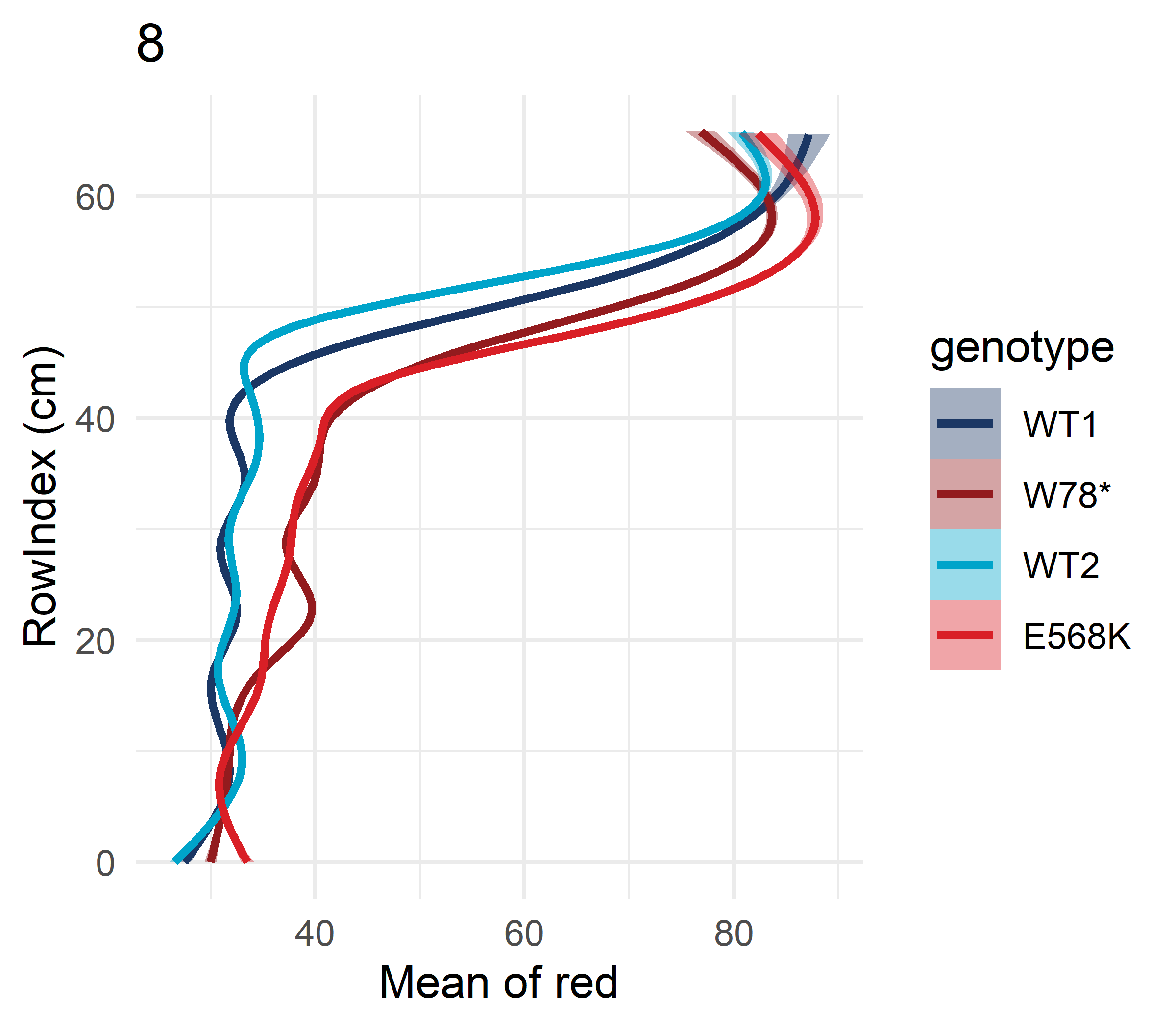
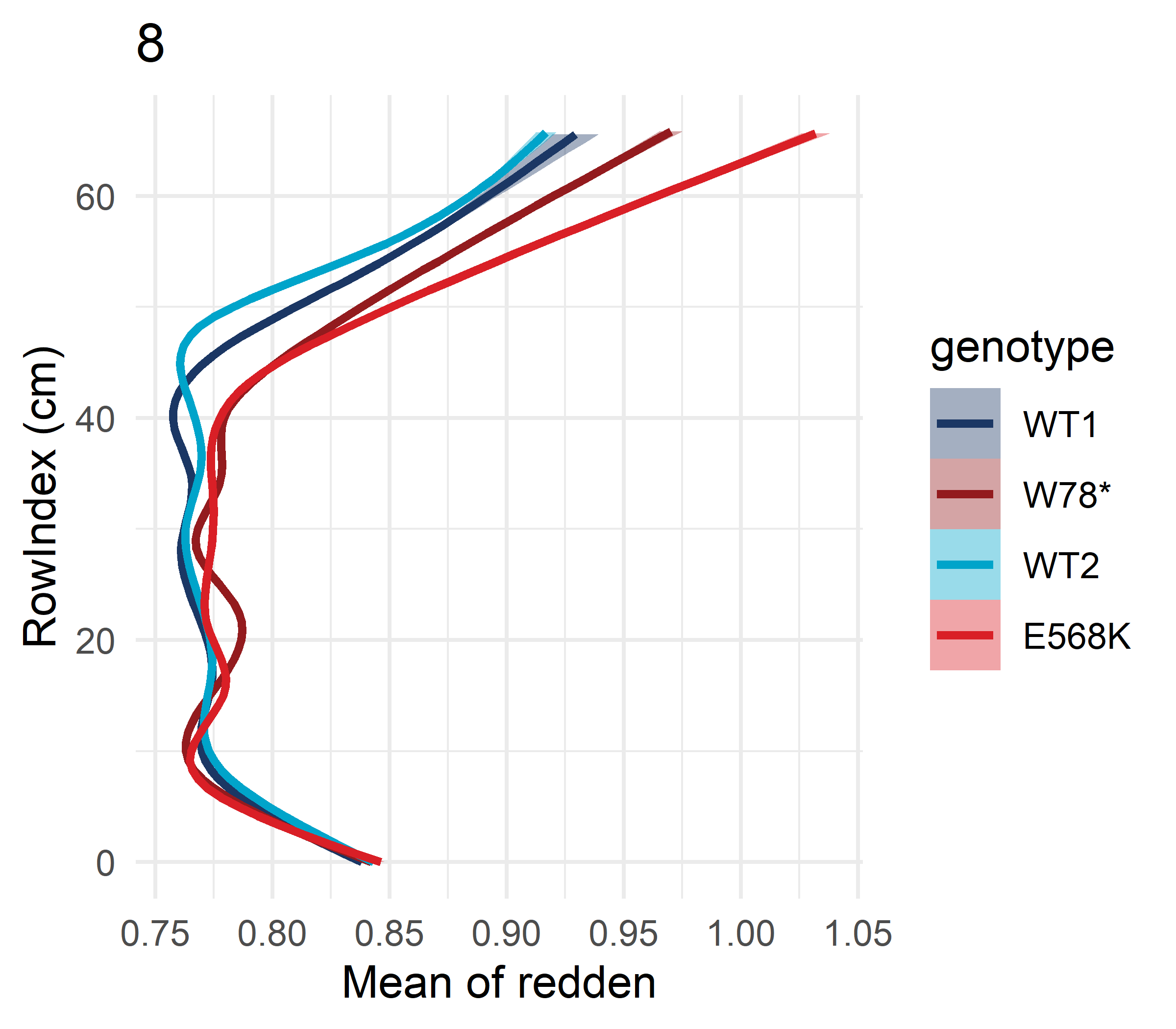
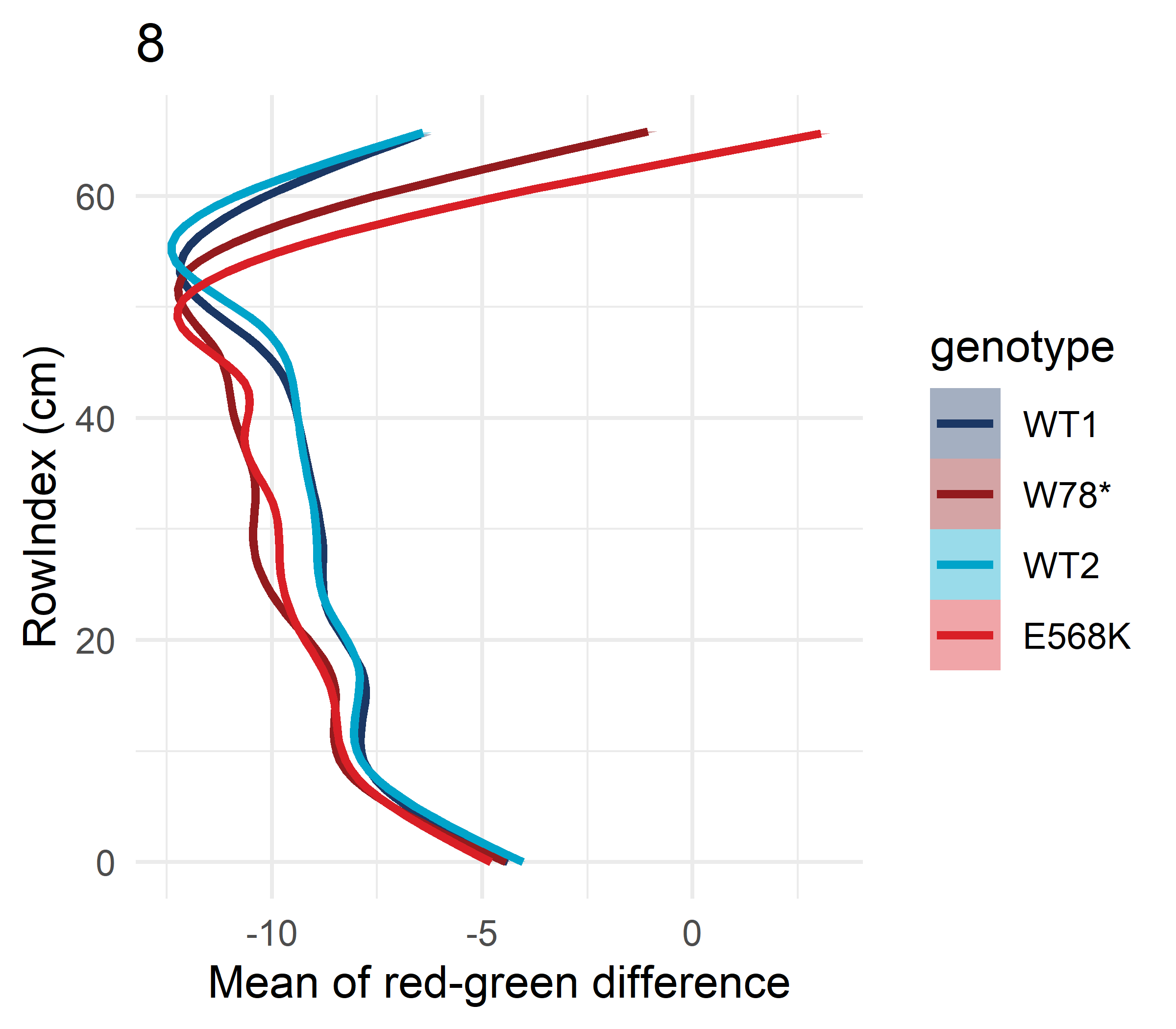
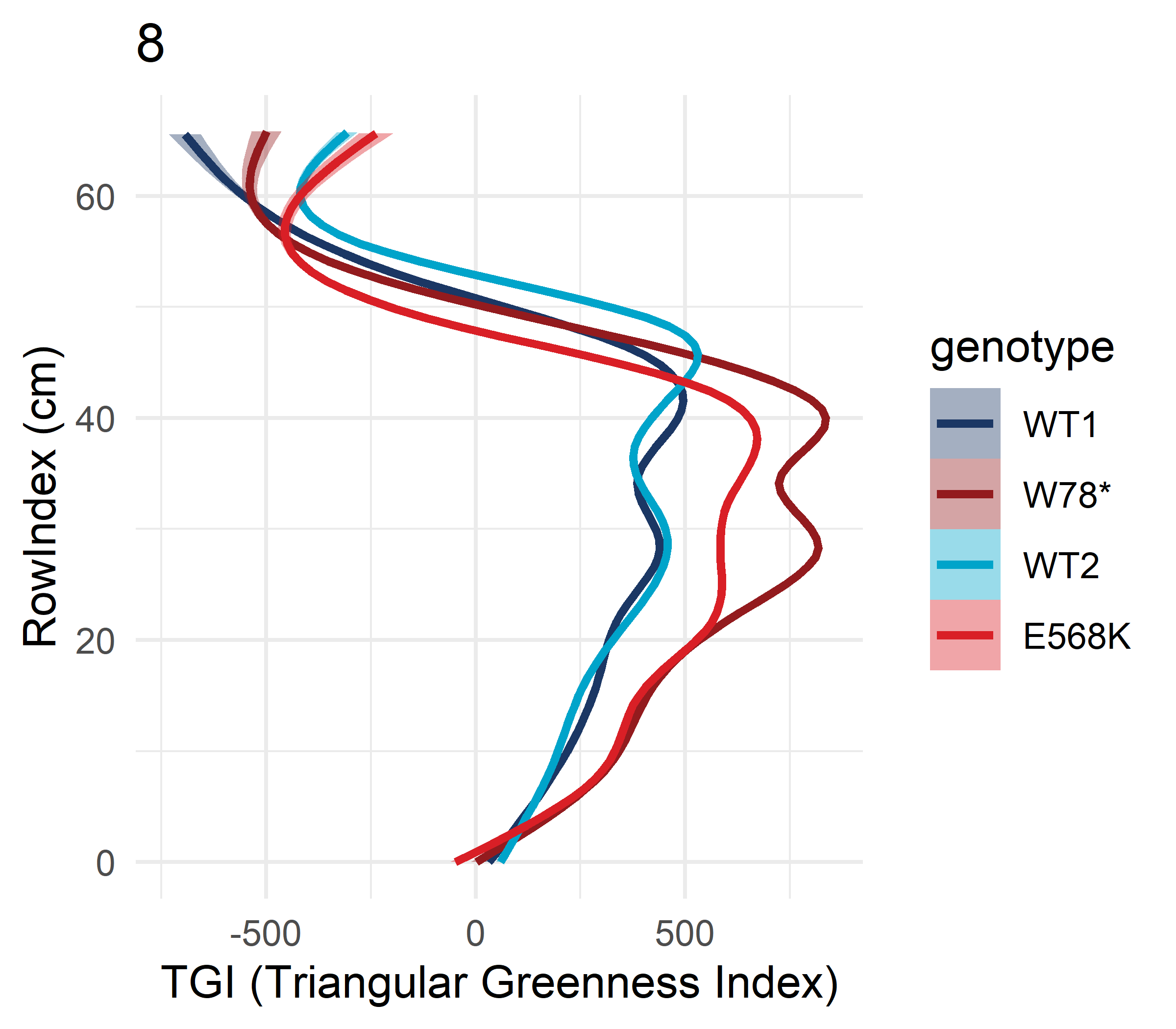
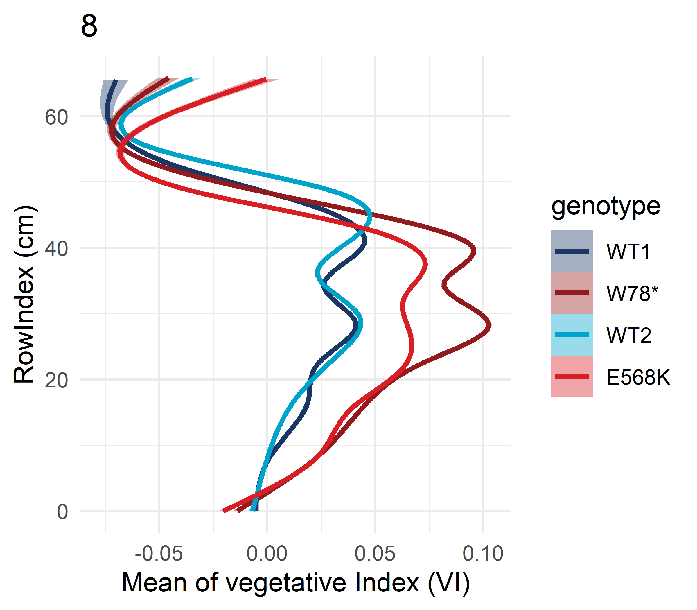
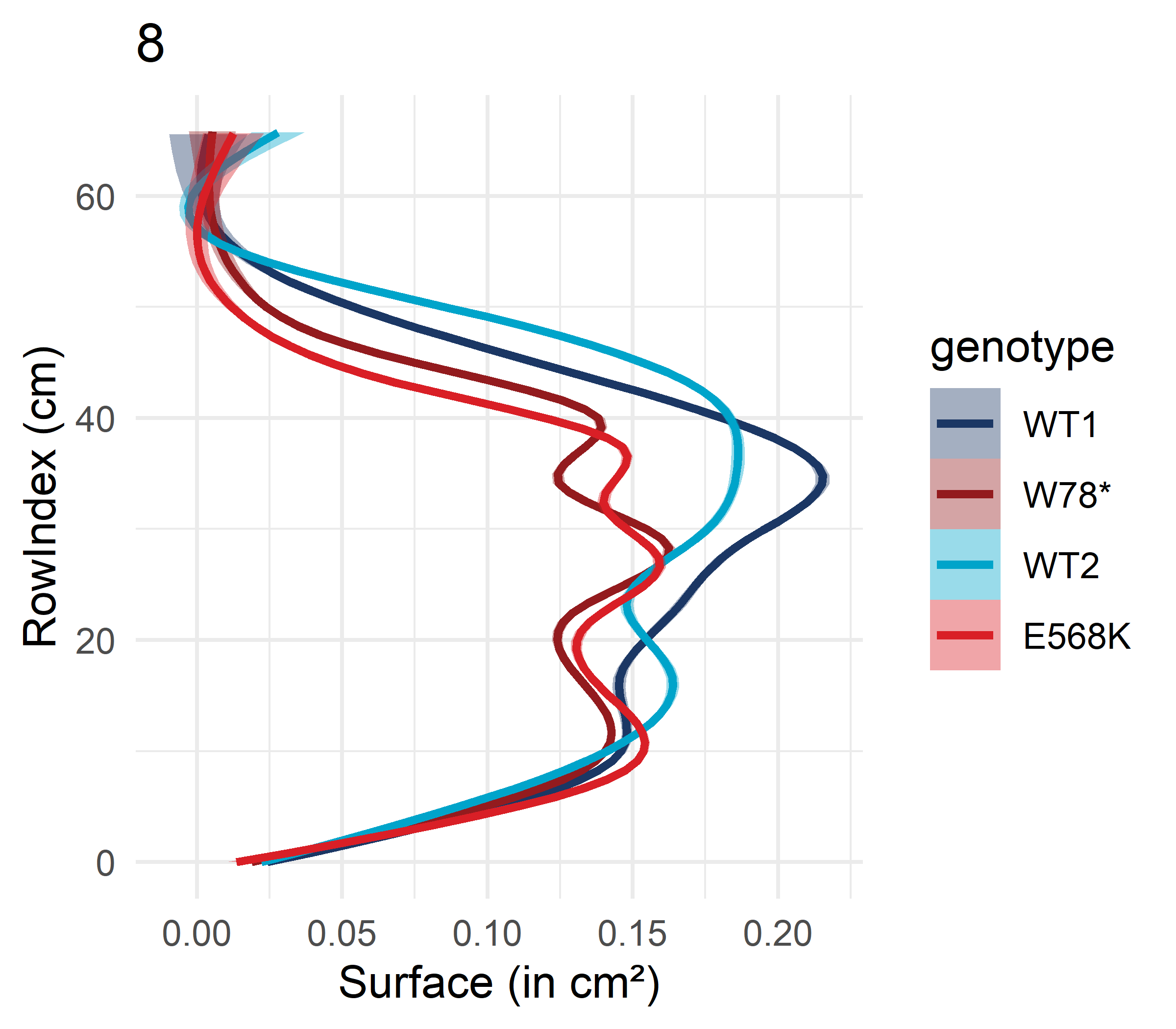
--- output: html_document editor_options: chunk_output_type: console resources: - py/TimeLapse_04_17_2025_10_05_14_crop.mp4 - py/TimeLapse_04_17_2025_10_06_45_segmented_crop.mp4 - py/TimeLapse_04_17_2025_10_10_43_extracted_crop.mp4 - py/TimeLapse_04_17_2025_10_08_13_convexhull.mp4 - py/TimeLapse_04_17_2025_10_19_34_RVB_crop.mp4 --- ## Plant phenotyping ```{r} #pkg library (tidyverse)library (here)library (readxl)library (ggh4x)library (ggstats)library (progressr)library (viridis) library (patchwork)library (ggplot2)# src source (here:: here ("src/function/stat_function/stat_analysis_main.R" )) # for make plot source (here:: here ("src/function/fig_export.R" )) # This function saves a given plot (plot_x) as both a PDF and a high-resolution PNG file at specified dimensions. # cosmetics = read_excel (here:: here ("data/color_palette.xlsm" )) %>% filter (set == "sulfure_condition" ) %>% :: select (color, treatment) %>% pull (color) %>% setNames (read_excel (here:: here ("data/color_palette.xlsm" )) %>% filter (set == "sulfure_condition" ) %>% pull (treatment)= read_excel (here:: here ("data/color_palette.xlsm" )) %>% filter (set == "mutant" ) %>% :: select (color, treatment) %>% pull (color) %>% setNames (read_excel (here:: here ("data/color_palette.xlsm" )) %>% filter (set == "mutant" ) %>% pull (treatment)``` - After phenotyping, put the correct plant name for each photo in the format `SHOOT_VIS_<SIDE/TOP>id_<plant_id>_name_GEAPS28_0325_ang_<imgangle>_date_<date_convertie>.png` - Create a model with ilastic to identify what is plant and what is not- Segment the image (plant vs. background) and put it in the `segmented` folder- Then a script convert the png image with 1 and 2 (corresponding to background and plant) into image compose of RGB (0,0,0) or (255,255,255). <a href="./py/convert_black_to_segmented.py" title="Download the Python script here"> <img src="py/python.ico" alt="Python" style="width: 24px; height: 24px;"/>For that is use this code</a>. - Then i tchek the number of pixel acording to the height to see were i can crop <a href="./py/plotting_black_pixcel.py" title="Download the Python script here"> <img src="py/python.ico" alt="Python" style="width: 24px; height: 24px;"/>with this code</a>.- Then I created an algorithm that slices the segmented image according to certain pixel heights to clean up pot or stake errors (below and above the plant). <a href="./py/correct_height_segmentation.py" title="Download the Python script here"> <img src="py/python.ico" alt="Python" style="width: 24px; height: 24px;"/>For that is use this code</a>. - Make a convex_hull with my old code. <a href="./py/measure_segmented_parameter.py" title="Download the Python script here"> <img src="py/python.ico" alt="Python" style="width: 24px; height: 24px;"/>See the code here</a>. - Then, we create background free image (plant withhout background) (in the folder `extracted` by using the previous image <a href="./py/extracted_plant.py" title="Download the Python script here"> <img src="py/python.ico" alt="Python" style="width: 24px; height: 24px;"/>with this code</a>- Then, We used this image to extract RGB features only from plant pixels- After segmenting the plant from the background, we computed color indices on the isolated plant region for all the plant. For that we use the folowing code <a href="./py/plant_RGB_measure.py" title="Download the Python script here"> <img src="py/python.ico" alt="Python" style="width: 24px; height: 24px;"/></a>- RGB ratios were calculated from plant-only masks to avoid background influence- We then did the same for each pixel of height of the plant (if, for example, it's greener for the lower parts than for the upper parts). For that we use the folowing code <a href="./py/plant_height_RGB_measure.py" title="Download the Python script here"> <img src="py/python.ico" alt="Python" style="width: 24px; height: 24px;"/></a>```{=html} <div style="display: flex; gap: 10px;"> <figure style="width: 33%; margin: 0; text-align: center;"> <figcaption style="margin-bottom: 5px; font-size: 1rem;">Original image</figcaption> <video src="py/TimeLapse_04_17_2025_10_05_14_crop.mp4" autoplay loop muted playsinline style="width: 100%; object-fit: cover;" > Votre navigateur ne supporte pas la balise <code>video</code>. </video> </figure> <figure style="width: 33%; margin: 0; text-align: center;"> <figcaption style="margin-bottom: 5px; font-size: 1rem;">Segmentation post deep learning algorithm</figcaption> <video src="py/TimeLapse_04_17_2025_10_06_45_segmented_crop.mp4" autoplay loop muted playsinline style="width: 100%; object-fit: cover;" > Votre navigateur ne supporte pas la balise <code>video</code>. </video> </figure> <figure style="width: 33%; margin: 0; text-align: center;"> <figcaption style="margin-bottom: 5px; font-size: 1rem;">Extraction of colour pixels only for what has been recognised as plant</figcaption> <video src="py/TimeLapse_04_17_2025_10_10_43_extracted_crop.mp4" autoplay loop muted playsinline style="width: 100%; object-fit: cover;" > Votre navigateur ne supporte pas la balise <code>video</code>. </video> </figure> </div> ``` ```{=html} <figure style="width: 100%; margin: 0; text-align: center;"> <figcaption style="margin-bottom: 5px; font-size: 1rem;">Measure with the convex shape of the height and width</figcaption> <video src="py/TimeLapse_04_17_2025_10_08_13_convexhull.mp4" autoplay loop muted playsinline style="width: 100%; object-fit: cover;" > Votre navigateur ne supporte pas la balise <code>video</code>. </video> </figure> ``` ```{=html} <figure style="width: 100%; margin: 0; text-align: center;"> <figcaption style="margin-bottom: 5px; font-size: 1rem;">Measurement of the green, red and blue pixel quantities for each image. </figcaption> <video src="py/TimeLapse_04_17_2025_10_19_34_RVB_crop.mp4" autoplay loop muted playsinline style="width: 100%; object-fit: cover;" > Votre navigateur ne supporte pas la balise <code>video</code>. </video> </figure> ``` ## Measurement to analyze post Python algorithm - Average plant area (with average for each angle)- Maximum plant area- Average convex plant area (with average for each angle)- Maximum convex plant area- Average plant height (with average for each angle)- Average plant width (with average for each angle)- Max width for each plant### Data importation ```{r, eval = F} # df_global <- read_csv(here::here("data/physio/phenotyping/result_black_pixel_corrected.csv"),show_col_types = FALSE) %>% # mutate(Label = str_remove(Label, "_Simple Segmentation_segmented$")) %>% # dplyr::rename(surface = BlackPixels) %>% # left_join(.,read_csv(here::here("data/physio/phenotyping/pixelwise_summary.csv"),show_col_types = FALSE) %>% # mutate(Label = str_remove(Label, "_extracted$")), by = "Label") %>% # left_join(., read_csv(here::here("data/physio/phenotyping/result_convex_hull.csv"),show_col_types = FALSE) %>% # mutate(Label = str_remove(Label, "_Simple Segmentation_segmented_cor$")) %>% # dplyr::rename(height = profondeur, # width = largeur) %>% # dplyr::select(-num_label), by = "Label") %>% # # extracte info from label # mutate( # id = str_extract(Label, "(?<=id_)\\d+"), # angle = str_extract(Label, "(?<=ang_)\\d+"), # timestamp = str_extract(Label, "(?<=date_)\\d{4}-\\d{2}-\\d{2}_\\d{2}-\\d{2}-\\d{2}"), # date = str_extract(timestamp, "^\\d{4}-\\d{2}-\\d{2}"), # time = str_extract(timestamp, "(?<=_)\\d{2}-\\d{2}-\\d{2}"), # plant_num = as.numeric(id)-1000 # ) %>% # # add info from excel # left_join(., read_excel(here::here("data/plant_info.xlsx"), col_names = T) %>% # dplyr::rename("position"= "tablar position"), by = "plant_num") %>% # relocate(plant_num, genotype, row, line, depodding, condition, id, angle, timestamp, date, time, .before = Label) %>% # mutate(genotype=fct_relevel(genotype, "WT1", "W78*", "WT2", "E568K")) %>% # filter(area>2000000) # # # export # write_csv(df_global, here::here("data/physio/phenotyping/df_global.csv")) ## répertoire racine phenotyping_dir <- here("data/physio/phenotyping/results/pea_raw_shoot_v2/GEAPS28_0325") ##############test phenotyping_dir_test <- here("data/physio/phenotyping/results/pea_raw_shoot_v2/GEAPS28_0325/38517/pixelwise_summary.csv") ###################### test test = read_csv(file = phenotyping_dir_test) as.numeric(test$MeanRGDiff[20:100]) ## petite fonction utilitaire ----------------------------------------------- read_phenotyping <- function(pattern) { # Récupère tous les fichier(s) qui correspondent au nom passé en argument, # dans n'importe quel sous-dossier (recursive = TRUE) list.files( phenotyping_dir, pattern = pattern, recursive = TRUE, full.names = TRUE ) |> map_dfr(~ read_csv(.x, show_col_types = FALSE) |> mutate(taskid = basename(dirname(.x)))) # optionnel : identifie la date/lot } read_phenotyping <- function(pattern) { list.files( phenotyping_dir, pattern = pattern, recursive = TRUE, full.names = TRUE ) |> purrr::map_dfr(~ { df <- readr::read_csv(.x, show_col_types = FALSE) # 1. change « , » -> « . » dans toutes les colonnes texte df <- dplyr::mutate( df, across(where(is.character), ~ stringr::str_replace_all(.x, ",", ".")) ) # 2. reconvertit automatiquement (nombres, dates, etc.) df <- readr::type_convert(df, locale = readr::locale(decimal_mark = ".")) # 3. ajoute l’identifiant de lot df$taskid <- basename(dirname(.x)) df }) } ## import identique ---------------------------------------------------------- df_black <- read_phenotyping("result_black_pixel_corrected\\.csv$") |> mutate(Label = str_remove(Label, "_Simple Segmentation_segmented$")) |> dplyr::rename(surface = BlackPixels) df_pixel <- read_phenotyping("pixelwise_summary\\.csv$") |> mutate(Label = str_remove(Label, "_extracted$")) df_convex <- read_phenotyping("result_convex_hull\\.csv$") |> mutate(Label = str_remove(Label, "_Simple Segmentation_segmented_cor$")) |> dplyr::rename(height = profondeur, width = largeur) |> dplyr::select(-num_label) ## import size px for each taskid df_px <- read_excel(here::here("data/physio/phenotyping/conversion_px_cm.xlsx"), col_names = TRUE) ## pipeline de fusion -------------------------------------------------------- df_global <- df_black |> left_join(df_pixel, by = c("Label", "taskid")) |> # ← ajoute batch left_join(df_convex, by = c("Label", "taskid")) |> # ← ajoute batch mutate( id = str_extract(Label, "(?<=id_)\\d+"), angle = str_extract(Label, "(?<=ang_)\\d+"), timestamp = str_extract(Label, "(?<=date_)\\d{4}-\\d{2}-\\d{2}_\\d{2}-\\d{2}-\\d{2}"), date = str_extract(timestamp, "^\\d{4}-\\d{2}-\\d{2}"), time = str_extract(timestamp, "(?<=_)\\d{2}-\\d{2}-\\d{2}"), plant_num = as.numeric(id) - 1000, plant_num = ifelse(plant_num == 9020,20, plant_num) ) |> left_join( read_excel(here("data/plant_info.xlsx"), col_names = TRUE) |> dplyr::rename(position = `tablar position`), by = "plant_num" ) |> relocate( plant_num, genotype, row, line, depodding, condition, id, angle, timestamp, date, time, .before = Label ) |> mutate(genotype = fct_relevel(genotype, "WT1", "W78*", "WT2", "E568K")) |> filter(area > 2e6) %>% filter(plant_num!= 6) %>% mutate(DAP = as.numeric(as.Date(date)-as.Date("2025-04-10"))) %>% mutate(taskid = as.integer(taskid)) %>% left_join(., df_px, by ="taskid") %>% mutate(surface_cm_2 = surface * h_px^2, perimeter_cm = perimeter * h_px, area_cm_2 = area * h_px^2, height_cm = height * h_px, width_cm = width * h_px) %>% mutate(depodding = ifelse(depodding %in% c("D", "FD"), "Pod removal", "Control")) #levels(as.factor(df_global$plant_num)) # export write_csv(df_global, here::here("data/physio/phenotyping/df_global.csv")) ``` ### Data representation #### Examples of interesting ratios to test - `G / (R + B)` Green index- `R / G` Reddening / senescence tendency- `G / (R + G + B)` Percentage of green in the image- `R - G` Red-green difference- `(G - R) / (G + R)` Normalized Green Red Difference Index (NGRDI) Good indicator of health or stress- `(G - B) / (G + B)` Vegetative Index (VI) Often used in simple cases- `-0.5 * [(190*(R-G)) - (120*(R-B))]` TGI (Triangular Greenness Index) Estimates chlorophyll without a spectrometer```{r, eval = F} df_global = read.csv(here::here("data/physio/phenotyping/df_global.csv"),dec = ",", ) %>% mutate(genotype=fct_relevel(genotype, "WT1", "W78*", "WT2", "E568K")) %>% mutate(across(c(height_cm, width_cm, surface_cm_2, MeanGI, MeanVI), ~ as.numeric (.x))) %>% mutate(depodding = as.factor(depodding), depodding = factor(depodding,levels = c("Control", "Pod removal"))) df_global %>% ggplot(aes(x = as.factor(plant_num), y = as.numeric(height_cm), fill = genotype)) + geom_boxplot()+ facet_grid(. ~ taskid)+ scale_color_manual(values = mutant_palette) + scale_fill_manual(values = mutant_palette) + theme(axis.text.x = element_text(angle = 0, hjust = 1)) df_global %>% ggplot(aes(x = as.factor(plant_num), y = MeanGI, fill = genotype)) + geom_boxplot()+ facet_grid(. ~ taskid)+ scale_color_manual(values = mutant_palette) + scale_fill_manual(values = mutant_palette) df_global %>% ggplot(aes(x = as.factor(plant_num), y = MeanVI, fill = genotype)) + geom_boxplot()+ facet_grid(. ~ taskid)+ scale_color_manual(values = mutant_palette) + scale_fill_manual(values = mutant_palette) cols_to_average <- c("surface_cm_2", "MeanR", "MeanG", "MeanB", "MeanGI", "MeanRedden", "MeanPctGreen", "MeanRGDiff", "MeanNGRDI", "MeanVI", "MeanTGI", "perimeter_cm", "area_cm_2", "height_cm", "width_cm") # remplace par tes vraies colonnes df_mean <- df_global %>% dplyr::group_by(plant_num, genotype, row, line, position, DAP, depodding) %>% dplyr::summarise( across( all_of(cols_to_average), list(mean = ~ mean(.x, na.rm = TRUE), sd = ~ sd(.x, na.rm = TRUE)), .names = "{.fn}_{.col}" ), .groups = "drop" ) %>% mutate( DAP_text = factor( paste0("DAP: ", DAP), levels = paste0("DAP: ", sort(unique(DAP))) ) ) %>% mutate(depodding = as.factor(depodding), depodding = factor(depodding,levels = c("Control", "Pod removal"))) # I take the most extreme value to measure the surface area of the plant. # juste for fun p_surface = df_mean %>% ggplot(aes(x = genotype, y = mean_surface_cm_2, fill = genotype, linetype = depodding)) + geom_boxplot(alpha = .6)+ facet_grid(. ~ DAP_text) + theme_bw()+ scale_color_manual(values = mutant_palette) + scale_fill_manual(values = mutant_palette)+ labs(fill = "Genotype")+ theme( axis.text.x = element_text(angle = 90, vjust = 0.5, size = 12), axis.text.y = element_text(size = 12), # axis.title = element_text(size = 14, face = "bold"), strip.text = element_text(size = 12), legend.position = "bottom", legend.title = element_text(size = 13), legend.text = element_text(size = 14) )+ labs(y = "Surface (cm²)", x = "Genotype", linetype = "Depodding") ; p_surface fig_export(here::here(paste0("report/physio/plot/phenotyping/cinetic_surface")),format= "png", p_surface, height_i = 7, width_i = 15, res_i = 600) df_mean %>% ggplot(aes(x = DAP, y = mean_surface_cm_2, color = genotype)) + geom_smooth(alpha = .2)+ theme_bw()+ scale_color_manual(values = mutant_palette) + labs(color = "Genotype", y = "Surface (cm²)") df_mean %>% ggplot(aes(x = DAP, y = mean_MeanVI, color = genotype)) + geom_smooth(alpha = .2)+ theme_bw()+ scale_color_manual(values = mutant_palette) + labs(color = "Genotype", y = "VI") df_global %>% dplyr::group_by(genotype, DAP) %>% dplyr::summarise( across( all_of(cols_to_average), list(mean = ~ mean(.x, na.rm = TRUE), sd = ~ sd(.x, na.rm = TRUE)), .names = "{.fn}_{.col}" ), .groups = "drop" ) %>% mutate( DAP_text = factor( paste0("DAP: ", DAP), levels = paste0("DAP: ", sort(unique(DAP))) ) ) %>% ggplot(aes(x = DAP, y = mean_surface_cm_2, color = genotype)) + geom_point(position = position_dodge(width = 2), size = 2) + geom_errorbar(aes(ymin = mean_surface_cm_2 - sd_surface_cm_2, ymax = mean_surface_cm_2 + sd_surface_cm_2), width = 1, position = position_dodge(width = 2)) + theme_bw(base_size = 12) + theme( legend.position = "bottom", axis.text.x = element_text(hjust = 1), panel.spacing = unit(0.5, "lines") )+ scale_color_manual(values = mutant_palette) df_mean %>% ggplot(aes(x = genotype, y = mean_MeanTGI, fill = genotype)) + geom_boxplot()+ facet_grid(. ~ DAP) + scale_color_manual(values = mutant_palette) + scale_fill_manual(values = mutant_palette) df_mean %>% mutate(DAP = as.numeric(as.character(DAP))) %>% ggplot(aes(x = DAP, y = mean_MeanTGI , color = genotype)) + geom_smooth(method = "loess", se = TRUE) + scale_color_manual(values = mutant_palette) + scale_x_continuous(breaks = unique(as.numeric(as.character(df_mean$DAP)))) + theme_bw(base_size = 12) + theme( legend.position = "bottom" )+labs(y= " ", color= "Genotype") mod1=lm(formula = mean_surface_cm_2 ~ genotype+row+as.factor(line)+as.factor(DAP), data = df_mean) p_x<-ggcoef_model(mod1) ; p_x col_variable = colnames(df_mean)[7:21] col_variable_legend = c("Surface", "Mean of red", "Mean of green", "Mean of blue", "Mean of green index", "Mean of redden", "Mean percentage of green in the image", "Mean of red-green difference", "Mean of normalized Green Red \nDifference Index (NGRDI)", "Mean of vegetative Index (VI)", "TGI (Triangular Greenness Index)", "Mean of of perimeter of the convexhull", "Mean of the area of the convexhull", "Mean of the height", "Mean of the width") for (date_i in levels(as.factor(df_mean$date))){ for (i in 1:length(col_variable)){ p <- stat_analyse( data=df_mean %>% filter(date == date_i) %>% as.data.frame() %>% mutate(genotype=fct_relevel(genotype, "WT1", "W78*", "WT2", "E568K")), #mutate(climat_condition=paste0(water_condition,"_",heat_condition)) %>% #mutate(condition=factor(condition,levels=c("Sto_WW_OT","Stoc_WS_OT","Sto_WW_HS","Sto_WS_HS","Wen_WW_OT","Wen_WS_OT","Wen_WW_HS","Wen_WS_HS"))) %>% column_value = col_variable[i], category_variables = c("genotype"), grp_var = "", show_plot = T, outlier_show = F, label_outlier = "plant_num", biologist_stats = T, Ylab_i = col_variable_legend[i], control_conditions = "", strip_normale = F, hex_pallet = mutant_palette ) p <-p[["plot"]]+labs(title = paste0(col_variable_legend[i]), subtitle = date_i, color="Genotype",fill="Genotype",x="Genotype") fig_export(here::here(paste0("report/physio/plot/phenotyping/",date_i,"_", col_variable[i])),format= "png", p, height_i = 3.5, width_i = 5, res_i = 600) } } ``` ```{r, echo=FALSE, results = "asis"} # ------------------------------------------------------------------- # Génère un tabset imbriqué : # niveau 1 = date (AAAA‑MM‑JJ) # niveau 2 = variable sans préfixe (ex. height, width, …) # ------------------------------------------------------------------- dir_plots <- "plot/phenotyping" # dossier des figures image_files <- list.files( path = dir_plots, pattern = "^\\d{4}-\\d{2}-\\d{2}_.+\\.png$", # ex. 2025-04-10_mean_height.png full.names = FALSE ) # --- extraire date et variable ------------------------------------- get_date <- function(x) sub("^([0-9]{4}-[0-9]{2}-[0-9]{2}).*$", "\\1", x) clean_var <- function(x) { x |> # pipe R ≥ 4.1 tools::file_path_sans_ext() |> sub("^\\d{4}-\\d{2}-\\d{2}_", "", x = _) |> # retire la date sub("^mean_", "", x = _) # retire mean_ } dates <- sort(unique(get_date(image_files))) # --- construire le markdown ---------------------------------------- tabset_code <- ":::: {.panel-tabset}\n\n" # niveau 1 for (d in dates) { tabset_code <- paste0(tabset_code, "## ", d, "\n\n", ":::: {.panel-tabset}\n\n") # niveau 2 # fichiers correspondant à la date courante files_d <- image_files[get_date(image_files) == d] for (file_name in files_d) { var_title <- clean_var(file_name) png_path <- file.path(dir_plots, file_name) html_path <- sub("\\.png$", ".html", png_path) tabset_code <- paste0( tabset_code, "### ", var_title, "\n\n", if (file.exists(html_path)) paste0("Version interactive : [Clique ici](", html_path, ")\n\n") else "", "\n\n" ) } tabset_code <- paste0(tabset_code, "::::\n\n") # fin niveau 2 } tabset_code <- paste0(tabset_code, "::::\n") # fin niveau 1 cat(tabset_code) ``` ## Green index as a function of plant height ### Data importation ```{r, eval = F} base_dir <- here("data/physio/phenotyping/results/pea_raw_shoot_v2/GEAPS28_0325") row_dirs_all <- list.dirs(base_dir, recursive = FALSE, full.names = TRUE) # Keep only the ones that contain a "rowwise_data" subfolder rowwise_dirs <- row_dirs_all %>% file.path("rowwise_data") %>% keep(dir.exists) ## ------------------------------------------------------------- ## 2. List all CSV files in those folders ## ------------------------------------------------------------- files <- rowwise_dirs %>% map(~ list.files(.x, pattern = "\\.csv$", full.names = TRUE)) %>% flatten_chr() ## ------------------------------------------------------------- ## 3. Read, bind, and process the data ## ------------------------------------------------------------- # activate progress bar all_data <- with_progress({ p <- progressor(along = files) map_dfr(files, function(f) { p(message = basename(f)) # mise à jour de la barre read.csv(f, stringsAsFactors = FALSE, dec = ",") %>% mutate(taskid = str_extract(f, "(?<=GEAPS28_0325/)[^/]+")) }) }) %>% mutate( Label = str_remove(Label, "_extracted$"), id = str_extract(Label, "(?<=id_)\\d+"), angle = str_extract(Label, "(?<=ang_)\\d+"), timestamp = str_extract(Label, "(?<=date_)\\d{4}-\\d{2}-\\d{2}_\\d{2}-\\d{2}-\\d{2}"), date = str_extract(timestamp, "^\\d{4}-\\d{2}-\\d{2}"), time = str_extract(timestamp, "(?<=_)\\d{2}-\\d{2}-\\d{2}"), plant_num = as.numeric(id) - 1000 ) %>% mutate(plant_num = ifelse(plant_num == 9020,20, plant_num)) %>% left_join( read_excel(here::here("data/plant_info.xlsx"), col_names = TRUE) %>% dplyr::rename(position = `tablar position`), by = "plant_num" ) %>% relocate( plant_num, genotype, row, line, depodding, condition, id, angle, timestamp, date, time, .before = Label ) %>% mutate(genotype = fct_relevel(genotype, "WT1", "W78*", "WT2", "E568K"))%>% filter(plant_num!= 6) df_px <- read_excel(here::here("data/physio/phenotyping/conversion_px_cm.xlsx"), col_names = TRUE) all_data = all_data %>% mutate(DAP = as.numeric(as.Date(date)-as.Date("2025-04-10"))) %>% mutate(taskid = as.integer(taskid)) %>% left_join(., df_px, by ="taskid") %>% mutate(RowIndex_cm = RowIndex * h_px, SurfacePixels_cm = SurfacePixels * h_px^2) # levels(as.factor(all_data$plant_num)) ## ------------------------------------------------------------- ## 5. Export the final combined dataset ## ------------------------------------------------------------- write_csv( all_data, here::here("data/physio/phenotyping/df_global_rowwise_data.csv") ) ``` ### Data representation ```{r, eval = F} df_rowwise <- read_csv(here::here("data/physio/phenotyping/df_global_rowwise_data.csv"), show_col_types = F) %>% mutate(genotype=fct_relevel(genotype, "WT1", "W78*", "WT2", "E568K")) %>% drop_na(MeanGI) # df_agg <- df_rowise %>% # dplyr::group_by(genotype, plant_num, RowIndex) %>% # dplyr::summarise(meanMeanTGI = mean(MeanTGI, na.rm = TRUE)) %>% # ungroup() df_recal <- df_rowwise %>% # <- your data frame dplyr::group_by(genotype, plant_num, DAP) %>% ## bottom-most row that still contains plant pixels mutate(maxRowIndexNonNA = max(RowIndex_cm[!is.na(MeanVI)], na.rm = TRUE)) %>% ## new coordinate: distance (in rows) *above* the bottom of the plant mutate(RowIndex0 = maxRowIndexNonNA - RowIndex_cm) %>% dplyr::ungroup() write_csv(df_recal, here::here("data/physio/phenotyping/df_global_rowwise_recal_data.csv")) cols_to_average <- c("MeanR", "MeanG", "MeanB", "MeanGI", "MeanRedden", "MeanPctGreen", "MeanRGDiff", "MeanNGRDI", "MeanVI", "MeanTGI", "SurfacePixels_cm") col_variable_legend = c("Mean of red", "Mean of green", "Mean of blue", "Mean of green index", "Mean of redden", "Mean percentage of green in the image", "Mean of red-green difference", "Mean of normalized Green Red \nDifference Index (NGRDI)", "Mean of vegetative Index (VI)", "TGI (Triangular Greenness Index)", "Surface (in cm²)") df_agg <- df_recal %>% dplyr::group_by(genotype, plant_num, DAP, RowIndex0) %>% dplyr::summarise(across(all_of(cols_to_average), ~ mean(.x, na.rm = TRUE), .names = "{.col}")) %>% ungroup() for (DAP_i in levels(as.factor(df_agg$DAP))){ for (i in 1:length(cols_to_average)){ df_agg_date <- df_agg %>% filter(DAP == DAP_i) p<- ggplot(df_agg_date, aes_string(x = "RowIndex0", y = cols_to_average[i], color = "genotype", fill = "genotype")) + geom_smooth() + #geom_point(size = .01, alpha=.2)+ # geom_point(size = 0.01, alpha = 0.2) # uncomment if you want points labs(x = "RowIndex (cm)", y = col_variable_legend[i], title = DAP_i) + scale_color_manual(values = mutant_palette) + scale_fill_manual(values = mutant_palette) + theme_minimal() + coord_flip() fig_export(here::here(paste0("report/physio/plot/phenotyping/height_", DAP_i, cols_to_average[i])),format= "png", p, height_i = 3.5, width_i = 4, res_i = 600) } } ``` ```{r, echo=FALSE, results = "asis"} # ------------------------------------------------------------------- # Build a two-level tabset from files such as # height_2025-04-18MeanPctGreen.png # ------------------------------------------------------------------- dir_plots <- "plot/phenotyping" # relative folder with the images image_files <- list.files( path = dir_plots, pattern = "^height_\\d{4}-\\d{2}-\\d{2}.+\\.png$", # new naming scheme full.names = FALSE ) image_files <- list.files( path = dir_plots, pattern = "^height_\\d.+\\.png$", full.names = FALSE ) # ----- helper functions -------------------------------------------- #get_date <- function(x) sub("^height_(\\d{4}-\\d{2}-\\d{2}).*$", "\\1", x) get_number <- function(x) sub("^height_(\\d+).*", "\\1", x) # clean_var <- function(x) { # x |> # tools::file_path_sans_ext() |> # drop ".png" # sub("^height_", "", x = _) |> # drop prefix # sub("^\\d{4}-\\d{2}-\\d{2}", "", x = _) |> # drop date # sub("^[-_]*", "", x = _) |> # remove any dash / underscore left # sub("(?i)^mean[-_]?", "", x = _, perl = TRUE) # drop Mean/mean_ # } clean_var <- function(x) { x |> tools::file_path_sans_ext() |> # enlève ".png" sub("^height_", "", x = _) |> # enlève le préfixe sub("^\\d+", "", x = _) |> # ← remplace la ligne "date" : supprime les chiffres sub("^[-_]*", "", x = _) |> # enlève tirets/underscores résiduels sub("(?i)^mean[-_]?", "", x = _, perl = TRUE) # enlève "Mean"/"mean_" } #dates <- sort(unique(get_date(image_files))) numbers <- sort(unique(get_number(image_files))) # ----- build the markdown code ------------------------------------- tabset_code <- ":::: {.panel-tabset}\n\n" # level 1 (date tabs) for (n in numbers) { tabset_code <- paste0( tabset_code, "## ", n, "\n\n", ":::: {.panel-tabset}\n\n" # level 2 (variable tabs) ) files_n <- image_files[get_number(image_files) == n] for (file_name in files_n) { var_title <- clean_var(file_name) png_path <- file.path(dir_plots, file_name) html_path <- sub("\\.png$", ".html", png_path) tabset_code <- paste0( tabset_code, "### ", var_title, "\n\n", if (file.exists(html_path)) paste0("[Interactive version](", html_path, ")\n\n") else "", "\n\n" ) } tabset_code <- paste0(tabset_code, "::::\n\n") # end level 2 } tabset_code <- paste0(tabset_code, "::::\n") # end level 1 cat(tabset_code) ``` ```{r, eval = F} df_recal <- read_csv(here::here("data/physio/phenotyping/df_global_rowwise_recal_data.csv")) for (date_i in levels(as.factor(df_recal$date))){ df_250_500 <- df_recal %>% filter(RowIndex0 >= 250, RowIndex0 <= 500) %>% # on garde la tranche d’intérêt dplyr::group_by(plant_num, genotype, row, line, position, date) %>% dplyr::summarise( mean_GI_250_500 = mean(MeanGI, na.rm = TRUE), # moyenne GI dans la tranche mean_VI_250_500 = mean(MeanVI, na.rm = TRUE), n_pixels = sum(!is.na(MeanGI)), # nb de lignes utilisées (optionnel) .groups = "drop" ) %>% filter(date == date_i) p <- stat_analyse( data=df_250_500 %>% as.data.frame() %>% mutate(genotype=fct_relevel(genotype, "WT1", "W78*", "WT2", "E568K")), #mutate(climat_condition=paste0(water_condition,"_",heat_condition)) %>% #mutate(condition=factor(condition,levels=c("Sto_WW_OT","Stoc_WS_OT","Sto_WW_HS","Sto_WS_HS","Wen_WW_OT","Wen_WS_OT","Wen_WW_HS","Wen_WS_HS"))) %>% column_value = "mean_GI_250_500", category_variables = c("genotype"), grp_var = "", show_plot = T, outlier_show = F, label_outlier = "plant_num", biologist_stats = T, Ylab_i = "Mean GI (250-500 px)", control_conditions = "", strip_normale = F, hex_pallet = mutant_palette ) p <-p[["plot"]]+labs(color="Genotype",fill="Genotype",x="Genotype", caption = date_i) fig_export(here::here(paste0("report/physio/plot/phenotyping/", date_i, "mean_GI_250-500_px")), format= "png", p, height_i = 3.5, width_i = 4, res_i = 600) } ``` # Green index (or VI) according to height and duration ```{r,eval = F} df_recal <- read_csv(here::here("data/physio/phenotyping/df_global_rowwise_recal_data.csv")) df_0_20 <- df_recal %>% filter(RowIndex0 >= 0, RowIndex0 <= 20) %>% # on garde la tranche d’intérêt dplyr::group_by(plant_num, genotype, row, line, position, date, DAP, depodding) %>% dplyr::summarise( mean_GI_250_500 = mean(MeanGI, na.rm = TRUE), # moyenne GI dans la tranche mean_VI_250_500 = mean(MeanVI, na.rm = TRUE), mean_TGI_250_500 = mean(MeanTGI, na.rm = TRUE), mean_R_250_500 = mean(MeanR, na.rm = TRUE), mean_G_250_500 = mean(MeanG, na.rm = TRUE), mean_B_250_500 = mean(MeanB, na.rm = TRUE), mean_G_B_250_500 = mean((MeanG/MeanB), na.rm = TRUE), mean_R_G_250_500 = mean((MeanR-MeanG), na.rm = TRUE), ExB = mean((2*MeanB-MeanR-MeanG), na.rm = TRUE), # 'indice anthocyane) ExG = mean((2*MeanG-MeanR-MeanB), na.rm = TRUE), # (vrai chlorose)() mean_MeanRedden_250_500 = mean(MeanRedden, na.rm = TRUE), n_pixels = sum(!is.na(MeanGI)), # nb de lignes utilisées (optionnel) .groups = "drop" ) %>% mutate(genotype=fct_relevel(genotype, "WT1", "W78*", "WT2", "E568K")) %>% mutate( depodding = ifelse( DAP > 22 & depodding %in% c("D", "FD"), # Check if date > 22 AND depodding is D or FD "Pod removal", "Control" # Otherwise, it's always "Control" ), depodding = as.factor(depodding), depodding = factor(depodding, levels = c("Control", "Pod removal")) ) df_20_40 <- df_recal %>% filter(RowIndex0 >= 20, RowIndex0 <= 40) %>% # on garde la tranche d’intérêt dplyr::group_by(plant_num, genotype, row, line, position, date, DAP, depodding) %>% dplyr::summarise( mean_GI_250_500 = mean(MeanGI, na.rm = TRUE), # moyenne GI dans la tranche mean_VI_250_500 = mean(MeanVI, na.rm = TRUE), mean_TGI_250_500 = mean(MeanTGI, na.rm = TRUE), mean_R_250_500 = mean(MeanR, na.rm = TRUE), mean_G_250_500 = mean(MeanG, na.rm = TRUE), mean_B_250_500 = mean(MeanB, na.rm = TRUE), mean_G_B_250_500 = mean((MeanG/MeanB), na.rm = TRUE), mean_R_G_250_500 = mean((MeanR-MeanG), na.rm = TRUE), ExB = mean((2*MeanB-MeanR-MeanG), na.rm = TRUE), # 'indice anthocyane) ExG = mean((2*MeanG-MeanR-MeanB), na.rm = TRUE), # (vrai chlorose)() mean_MeanRedden_250_500 = mean(MeanRedden, na.rm = TRUE), n_pixels = sum(!is.na(MeanGI)), # nb de lignes utilisées (optionnel) .groups = "drop" ) %>% mutate(genotype=fct_relevel(genotype, "WT1", "W78*", "WT2", "E568K")) %>% mutate( depodding = ifelse( DAP > 22 & depodding %in% c("D", "FD"), # Check if date > 22 AND depodding is D or FD "Pod removal", "Control" # Otherwise, it's always "Control" ), depodding = as.factor(depodding), depodding = factor(depodding, levels = c("Control", "Pod removal")) ) ###### tesrt ########## df_250_500 %>% ggplot(., aes(x= as.factor(DAP), y=mean_VI_250_500, col = genotype))+ geom_boxplot() #smooth df_250_500 %>% ggplot(., aes(x= DAP, y=mean_VI_250_500, col = genotype))+ geom_smooth() df_250_500 %>% ggplot(., aes(x= DAP, y=mean_GI_250_500, col = genotype))+ geom_smooth() df_250_500 %>% ggplot(., aes(x= DAP, y=mean_R_250_500, col = genotype))+ geom_smooth() df_250_500 %>% ggplot(., aes(x= DAP, y=mean_G_250_500, col = genotype))+ geom_smooth() df_250_500 %>% ggplot(., aes(x= DAP, y=mean_B_250_500, col = genotype))+ geom_smooth() df_250_500 %>% ggplot(., aes(x= DAP, y=mean_G_B_250_500, col = genotype))+ geom_smooth() df_250_500 %>% ggplot(., aes(x= DAP, y=mean_R_G_250_500, col = genotype))+ geom_smooth() df_250_500 %>% ggplot(., aes(x= DAP, y=ExB, col = genotype))+ geom_smooth() df_250_500 %>% ggplot(., aes(x= DAP, y=ExG, col = genotype))+ geom_smooth() ###### tesrt ########## #### scenecence ####### p_reeden <- df_0_20 %>% ggplot(., aes(x= DAP, y=mean_MeanRedden_250_500, col = genotype, linetype = depodding))+ geom_smooth(method = "loess", se = TRUE, alpha=0.2) + scale_color_manual(values = mutant_palette) + scale_x_continuous(breaks = unique(as.numeric(as.character(df_250_500$DAP)))) + geom_vline(xintercept=c(46), linetype="dotted", linewidth = 1.2)+ theme_bw(base_size = 12) + theme( legend.position = "right" ) + labs( y = "Reddening / senescence tendency \n(R / G) (at 0-20cm)", color = "Genotype", linetype = "Depodding" ) ; p_reeden #### Anthocianine ####### p_blue <- df_20_40 %>% ggplot(., aes(x= DAP, y=mean_G_B_250_500, col = genotype, linetype = depodding))+ geom_smooth(method = "loess", se = TRUE, alpha=0.2) + scale_color_manual(values = mutant_palette) + scale_x_continuous(breaks = unique(as.numeric(as.character(df_250_500$DAP)))) + geom_vline(xintercept=c(8), linetype="dotted", linewidth = 1.2)+ theme_bw(base_size = 12) + theme( legend.position = "right" ) + labs( y = "Intensity of blue color \n (G / B) (at 20-40cm)", color = "Genotype", linetype = "Depodding" ) ;p_blue # Montrer le pique d'Anthociane et l'augmentation de la couleur rouge. final_plot_cinetic <- (p_blue + p_reeden) + plot_layout(guides = "collect") & theme(legend.position = "bottom")& plot_annotation(tag_levels = "A") ; final_plot_cinetic # create boxplot behind p_stat_reeden <- stat_analyse( data=df_0_20 %>% as.data.frame() %>% filter(DAP == 41) %>% mutate(genotype=fct_relevel(genotype, "WT1", "W78*", "WT2", "E568K")), #mutate(climat_condition=paste0(water_condition,"_",heat_condition)) %>% #mutate(condition=factor(condition,levels=c("Sto_WW_OT","Stoc_WS_OT","Sto_WW_HS","Sto_WS_HS","Wen_WW_OT","Wen_WS_OT","Wen_WW_HS","Wen_WS_HS"))) %>% column_value = "mean_MeanRedden_250_500", category_variables = "depodding", grp_var = "genotype", show_plot = T, outlier_show = F, label_outlier = "plant_num", biologist_stats = T, Ylab_i = "Mean Reeden (at 0-20cm)", control_conditions = "", strip_normale = T#, #hex_pallet = "" ) p_stat_reeden <-p_stat_reeden[["plot"]]+labs(color="Genotype",fill="Genotype",x="Genotype") df_0_20_modif <- df_0_20 %>% as.data.frame() %>% filter(DAP == 41) %>% mutate(genotype=fct_relevel(genotype, "WT1", "W78*", "WT2", "E568K"), geno_depod = paste(sep = "_", genotype, depodding), geno_depod = as.factor(geno_depod), geno_depod=fct_relevel(geno_depod, "WT1_Control","WT1_Pod removal", "W78*_Control","W78*_Pod removal", "WT2_Control", "WT2_Pod removal","E568K_Control","E568K_Pod removal") ) %>% mutate( letter = case_when( geno_depod == "WT1_Control" ~ "ab", geno_depod == "WT1_Pod removal" ~ "a", geno_depod == "W78*_Control" ~ "bc", geno_depod == "W78*_Pod removal" ~ "bc", geno_depod == "WT2_Control" ~ "a", geno_depod == "WT2_Pod removal" ~ "ab", geno_depod == "E568K_Control" ~ "c", geno_depod == "E568K_Pod removal" ~ "c", TRUE ~ "" # Au cas où il y aurait d'autres génotypes non gérés ) ) letter_positions <- df_0_20_modif %>% group_by(genotype, depodding, geno_depod, letter) %>% summarise( # Trouvez la valeur Y maximale pour chaque boîte (genotype x depodding) y_max_box = max(mean_MeanRedden_250_500, na.rm = TRUE), .groups = 'drop' ) %>% # Ajoutez une marge au-dessus de la boîte. # La marge peut être un pourcentage de la hauteur totale du graphique ou une valeur fixe. # Utilisons un facteur pour la marge. mutate(y_pos_letter = y_max_box + (max(df_0_20_modif$mean_MeanRedden_250_500, na.rm = TRUE) * 0.03)) %>% # Ajustez le 0.03 si besoin # Ajoutez un décalage en X pour séparer les lettres "Control" et "Pod removal" mutate( x_offset = case_when( depodding == "Control" ~ -0.15, # Décalage léger à gauche pour 'Control' depodding == "Pod removal" ~ 0.15, # Décalage léger à droite pour 'Pod removal' TRUE ~ 0 # Par défaut (si d'autres types existaient) ) ) p_stat_reeden <- df_0_20_modif %>% ggplot(., aes(x=genotype, y = mean_MeanRedden_250_500, col= genotype,fill= genotype, linetype = depodding))+ geom_boxplot(outlier.alpha = 0, alpha = .25)+ geom_jitter(alpha=0.5,position = position_jitter(seed = 1),shape=16)+ scale_color_manual(values = mutant_palette) + scale_fill_manual(values = mutant_palette) + geom_vline(xintercept=c(8), linetype="dotted", linewidth = 1.2)+ theme_bw(base_size = 12) + theme( legend.position = "none" ) + labs( y = "Reddening / senescence tendency \n(R / G) (at 0-20cm and 41 DAP", y = "Genotype", color = "Genotype", fill = "Genotype", linetype = "Depodding" ) + geom_text(data = letter_positions, aes(x = as.numeric(genotype) + x_offset, # Positionne sur l'axe X avec le décalage y = 1.03*max(y_max_box), # Positionne sur l'axe Y au-dessus de la boîte label = letter, color = genotype), # Assure la couleur par génotype inherit.aes = FALSE, # Important pour ne pas hériter 'linetype' etc. size = 4, # Taille du texte vjust = 0.5, # Ajustement vertical hjust = 0.5) ; p_stat_reeden p_stat_blue <- stat_analyse( data=df_20_40 %>% as.data.frame() %>% filter(DAP == 8) %>% mutate(genotype=fct_relevel(genotype, "WT1", "W78*", "WT2", "E568K")), #mutate(climat_condition=paste0(water_condition,"_",heat_condition)) %>% #mutate(condition=factor(condition,levels=c("Sto_WW_OT","Stoc_WS_OT","Sto_WW_HS","Sto_WS_HS","Wen_WW_OT","Wen_WS_OT","Wen_WW_HS","Wen_WS_HS"))) %>% column_value = "mean_G_B_250_500", category_variables = "genotype", grp_var = "", show_plot = T, outlier_show = F, label_outlier = "plant_num", biologist_stats = T, Ylab_i = "Mean Blue (at 20-40cm at 8 DAP)", control_conditions = "", strip_normale = F, hex_pallet = mutant_palette ) p_stat_blue8 <-p_stat_blue[["plot"]]+labs(color="Genotype",fill="Genotype",x="Genotype")+theme_bw()+ theme(legend.position = "none") p_surface_bis = p_surface + theme(legend.position = "none") final_plot_global <-p_surface_bis/(p_blue + p_reeden)/(p_stat_blue8+p_stat_reeden) + plot_layout(guides = "collect") & theme(legend.position = "none")& plot_annotation(tag_levels = "A") ; final_plot_global fig_export(here::here(paste0("report/physio/plot/phenotyping/FigX_pheno")), final_plot_global, height_i = 12, width_i = 15, res_i = 600) ```