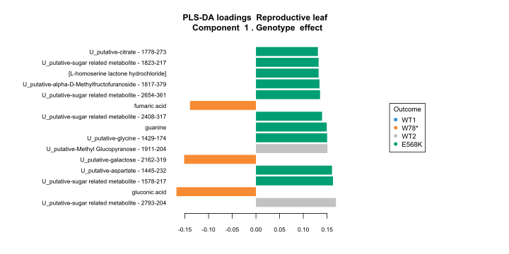
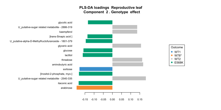
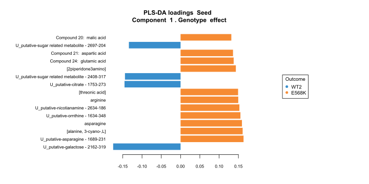
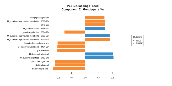
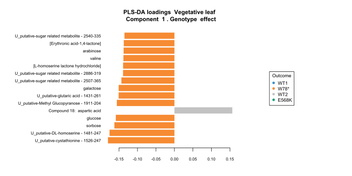
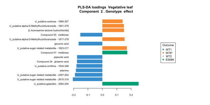
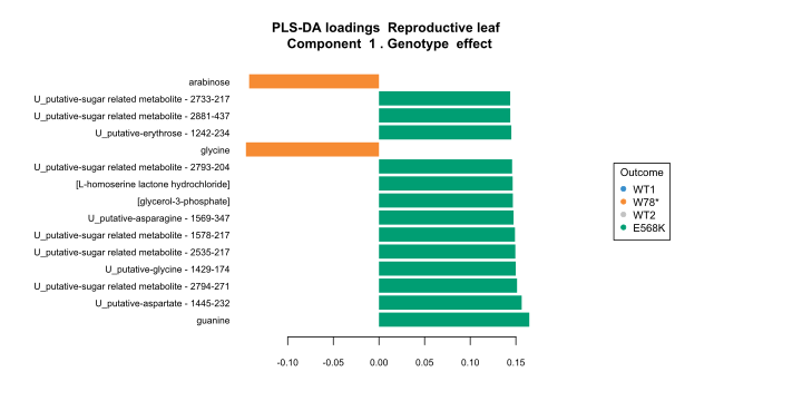
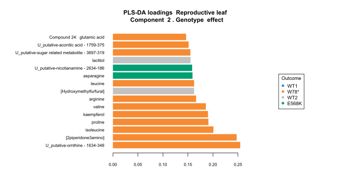
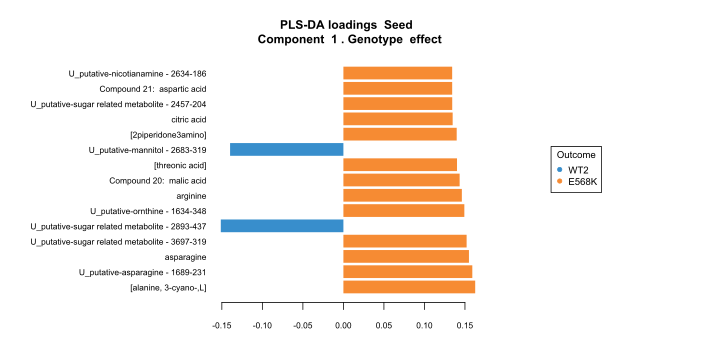
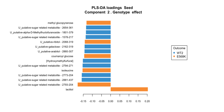
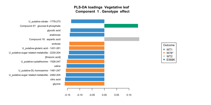
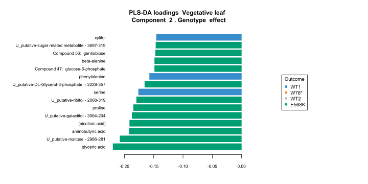
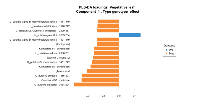
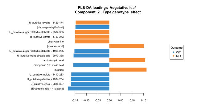
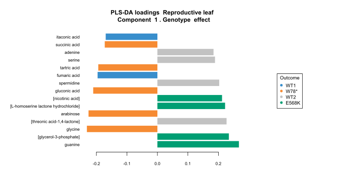
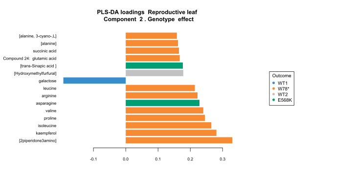
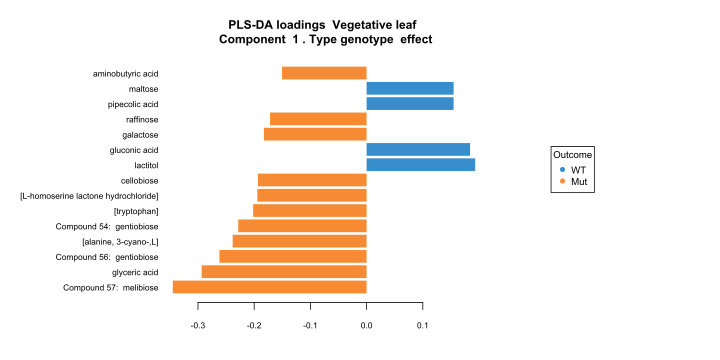
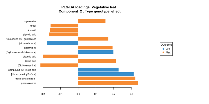
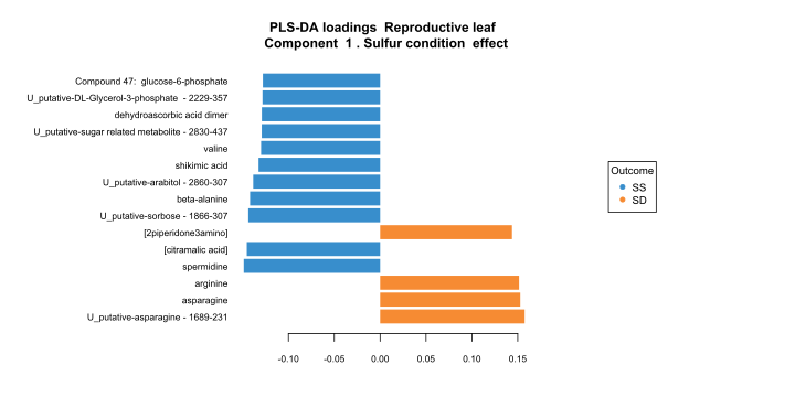
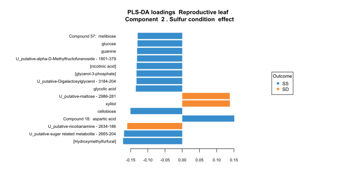
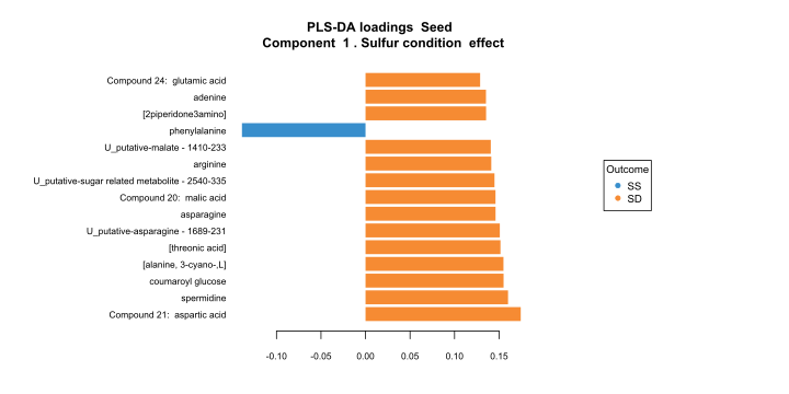
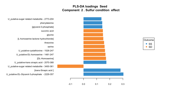
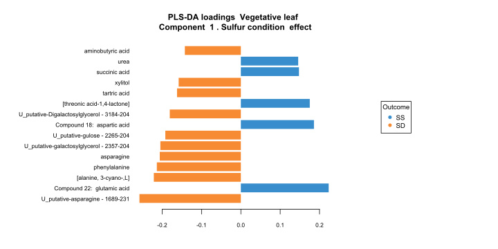
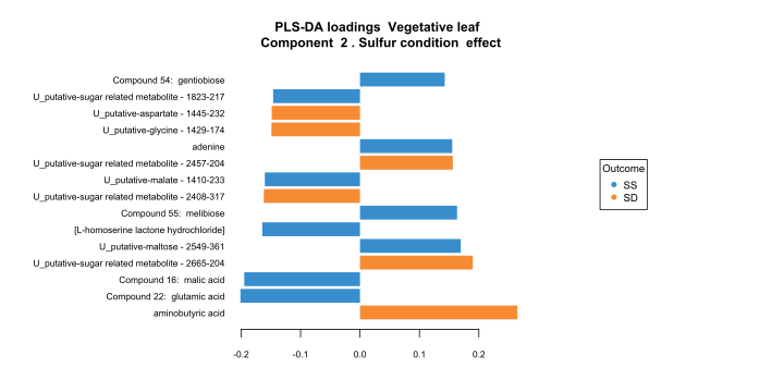
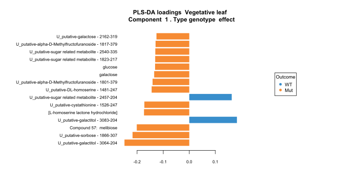
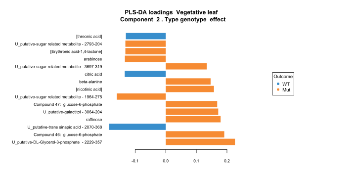
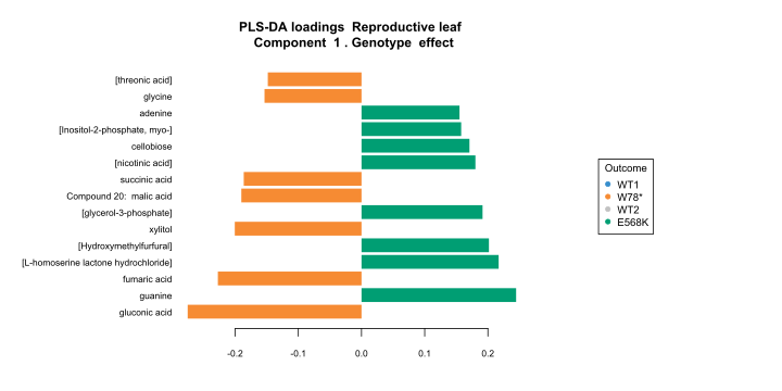
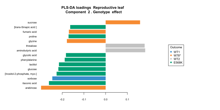
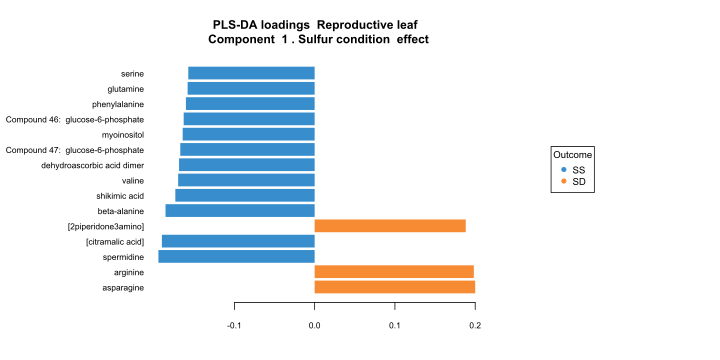
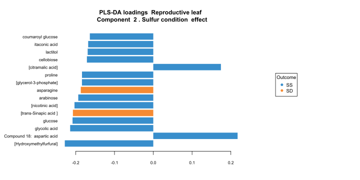
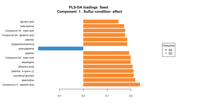
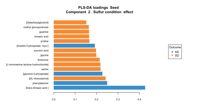
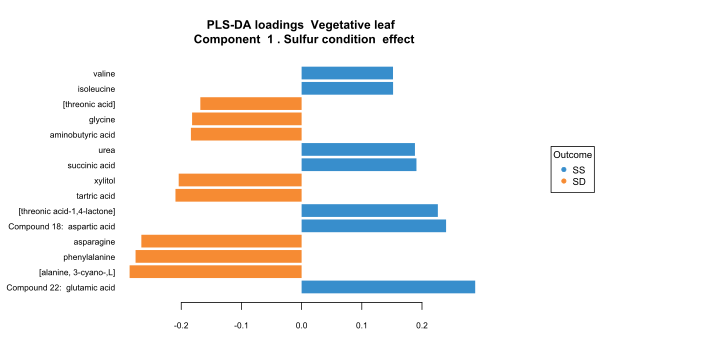
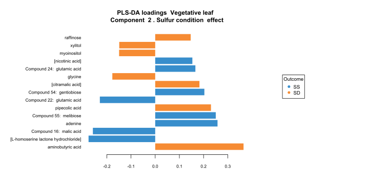
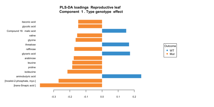
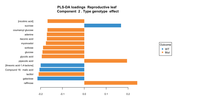
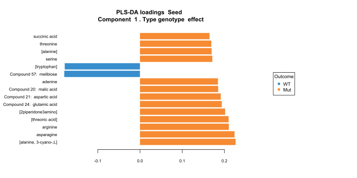
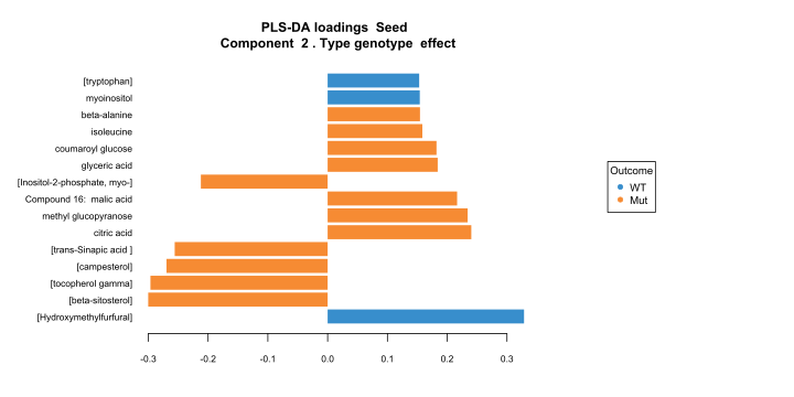
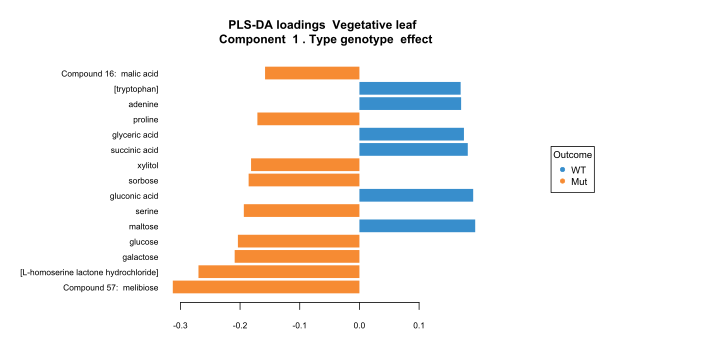
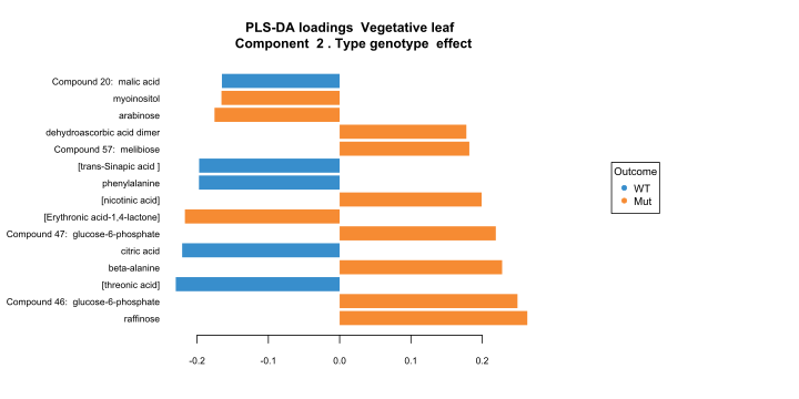
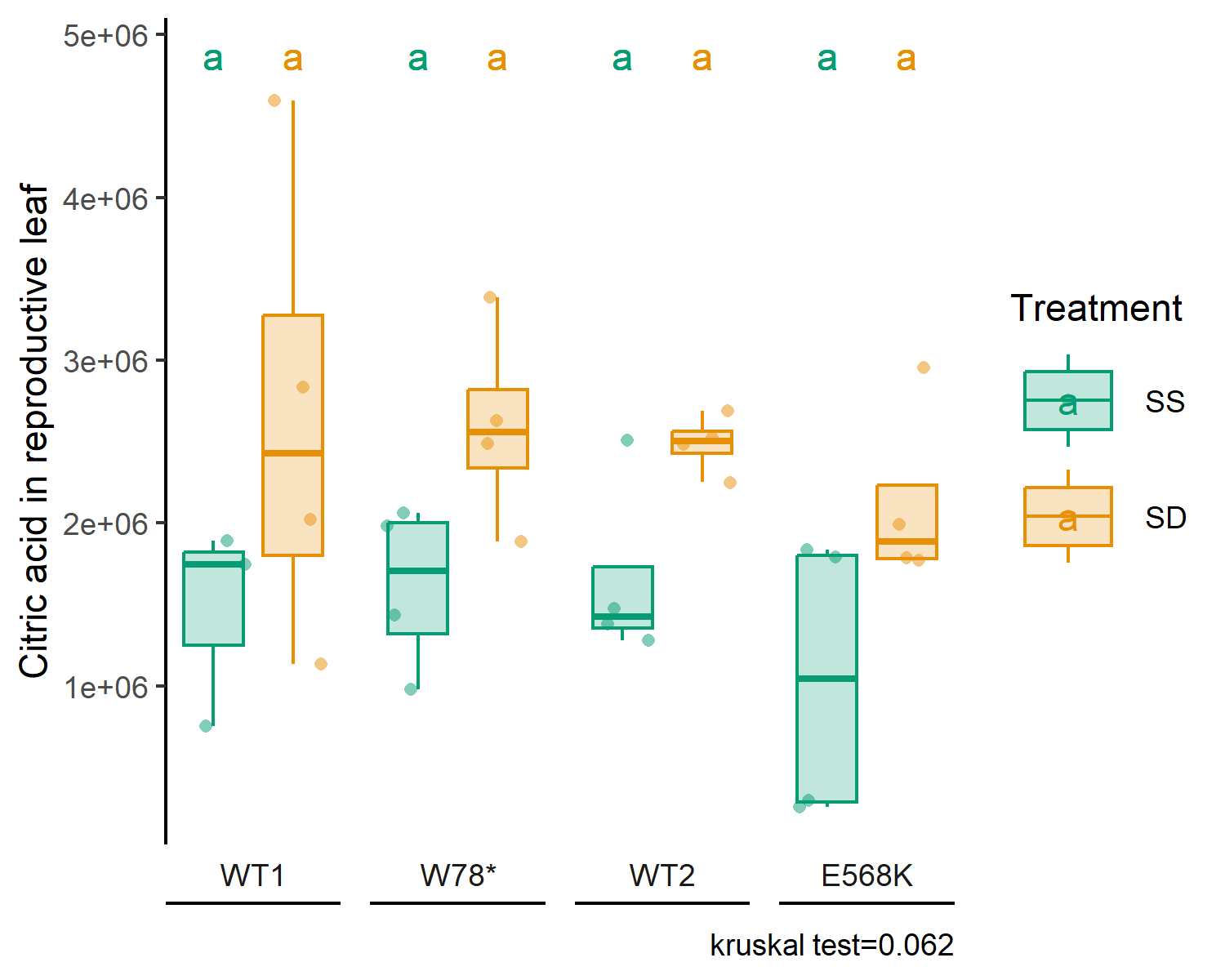
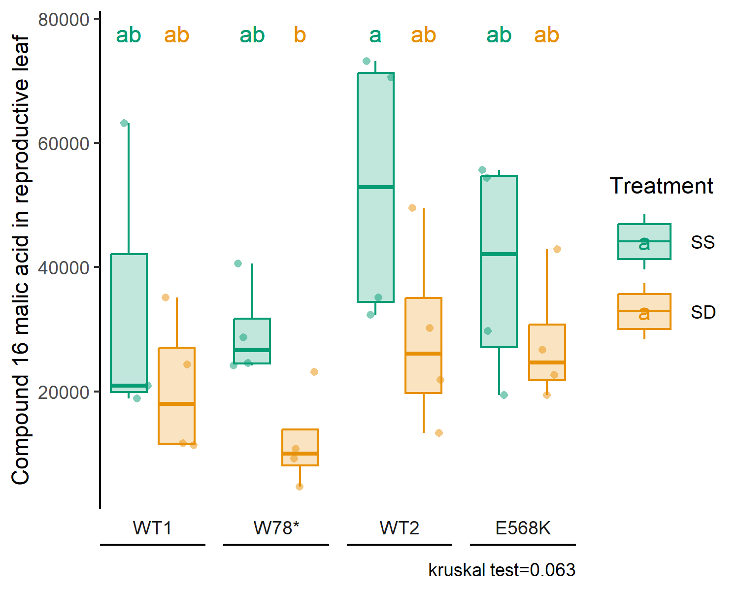
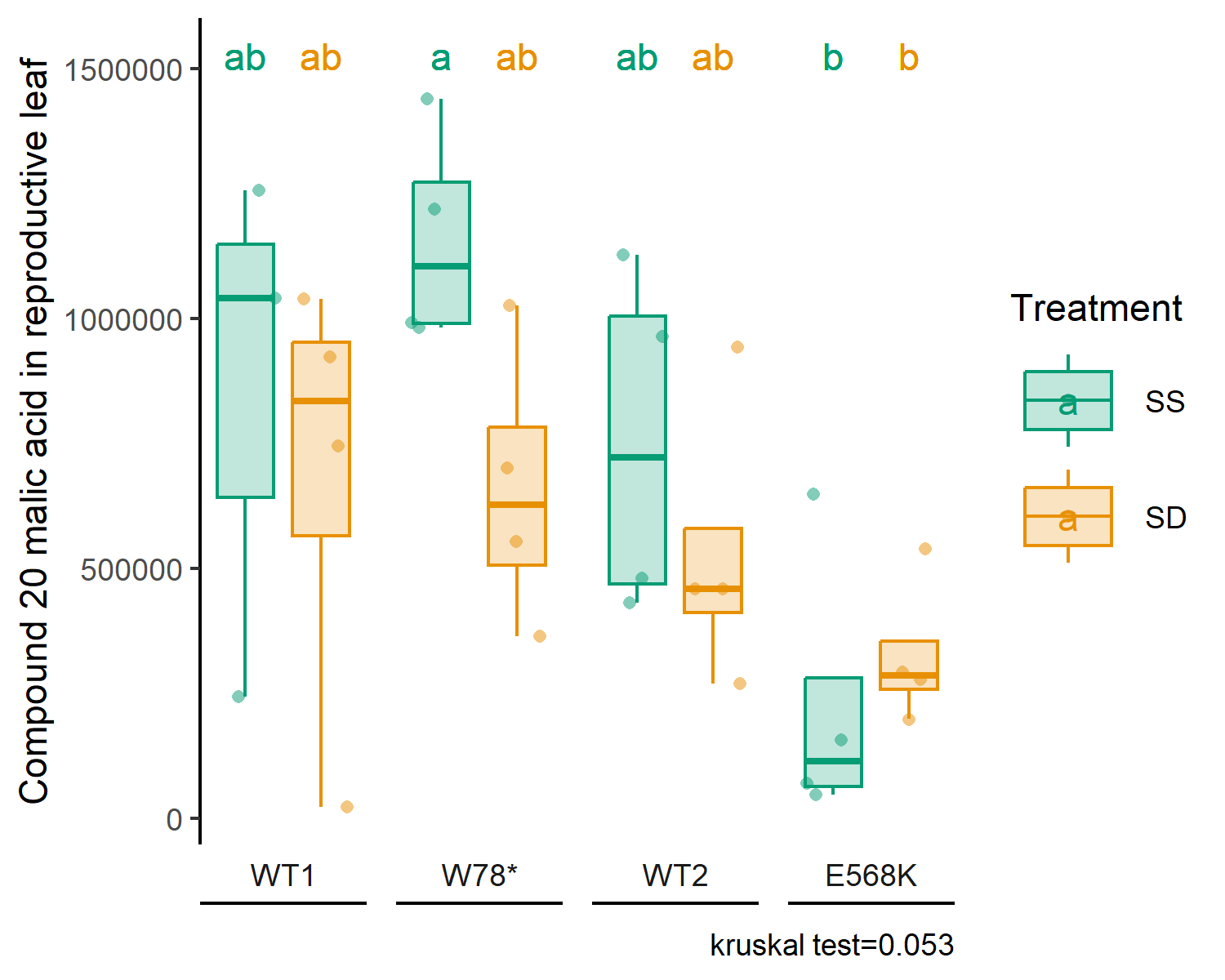
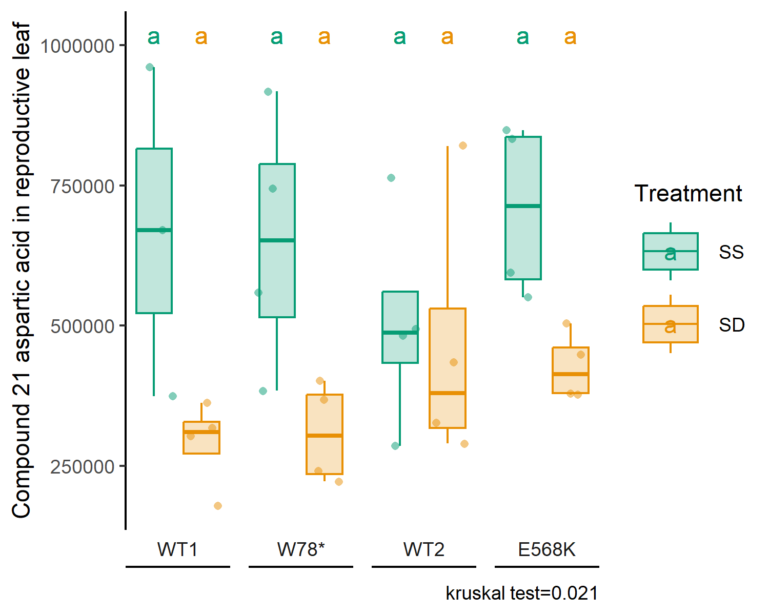
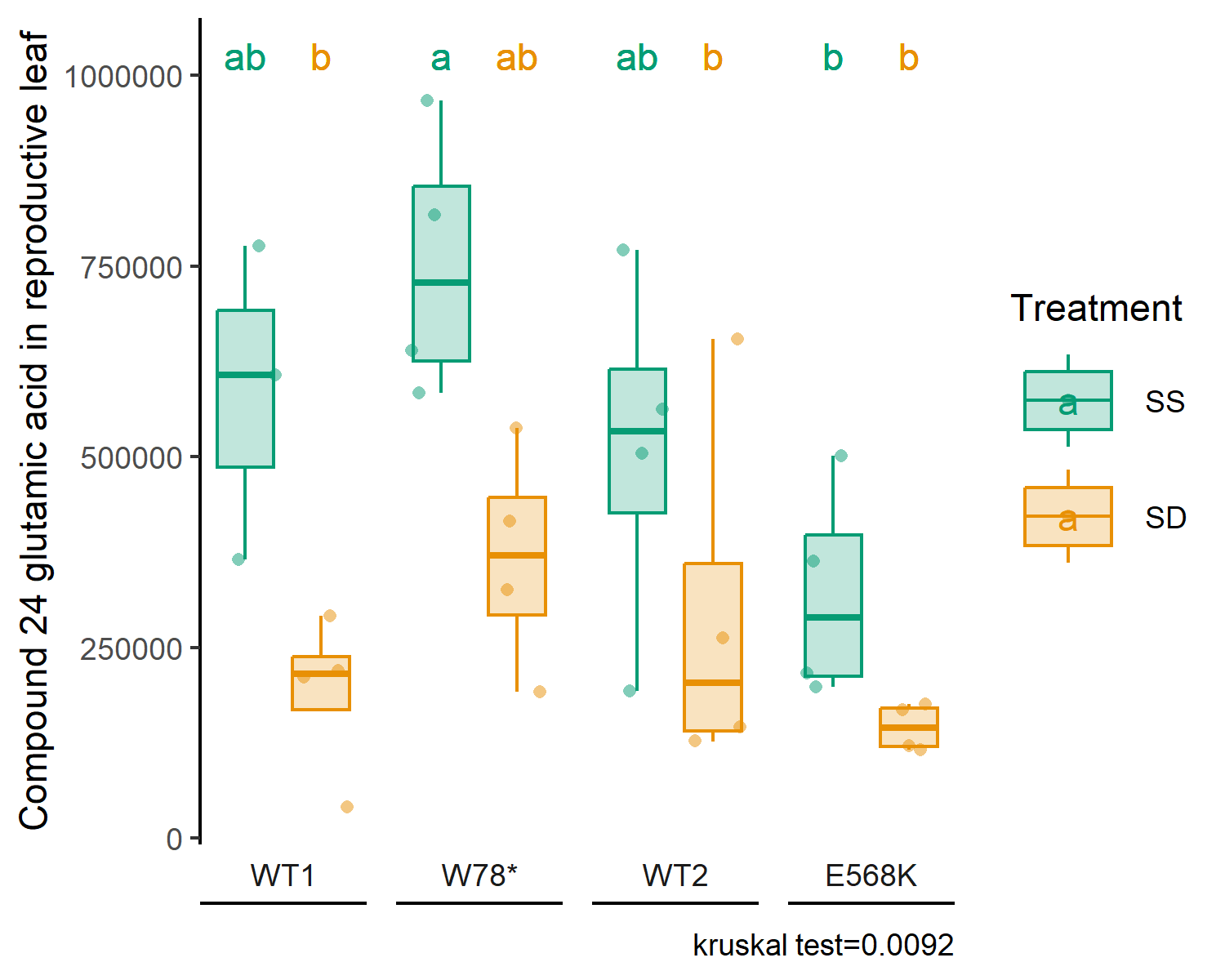
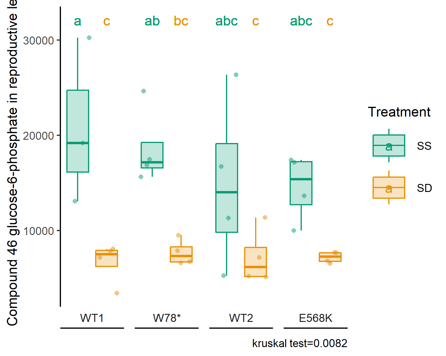
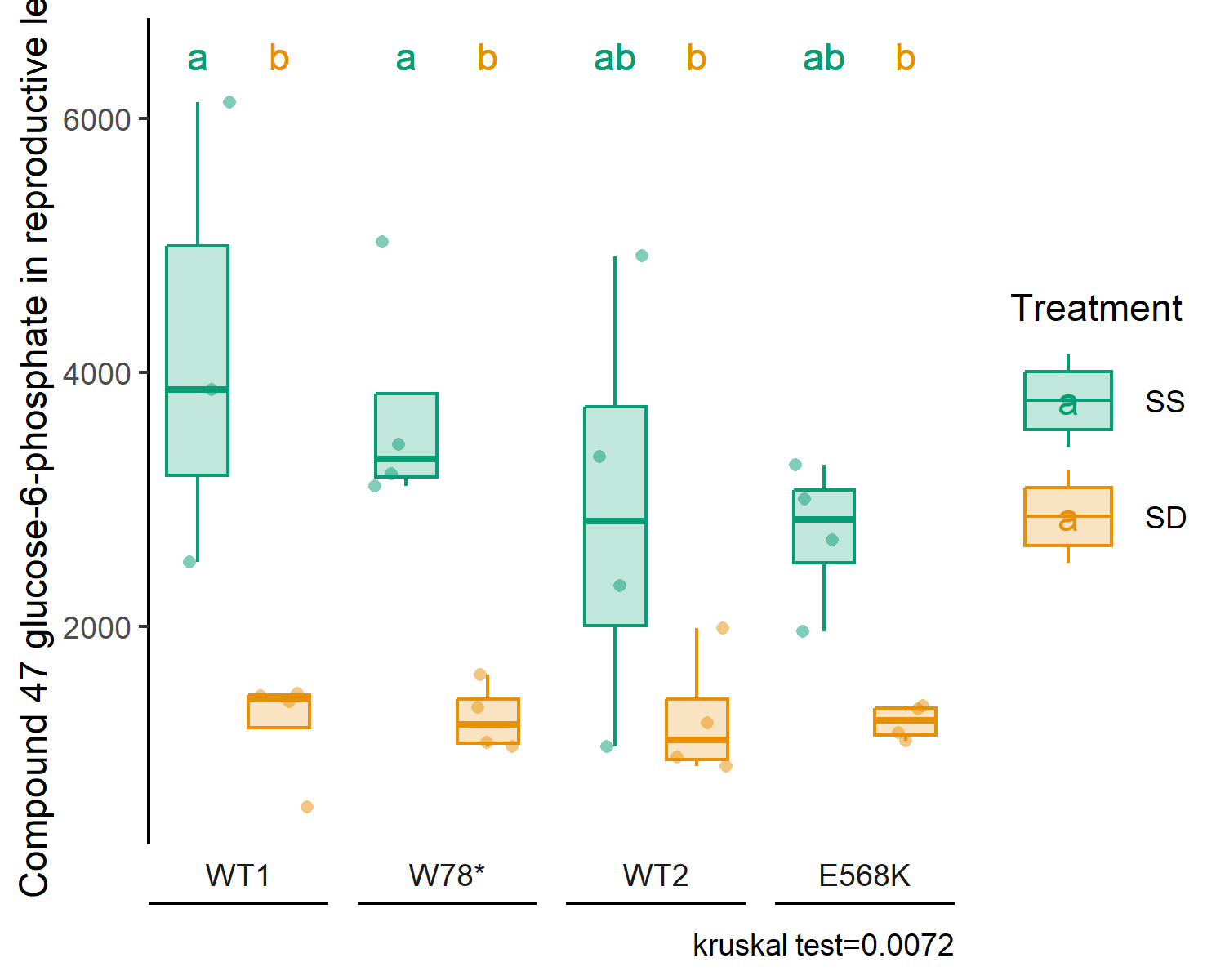
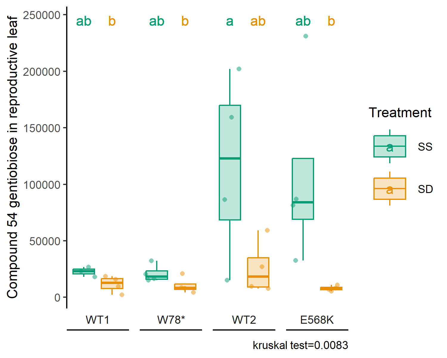
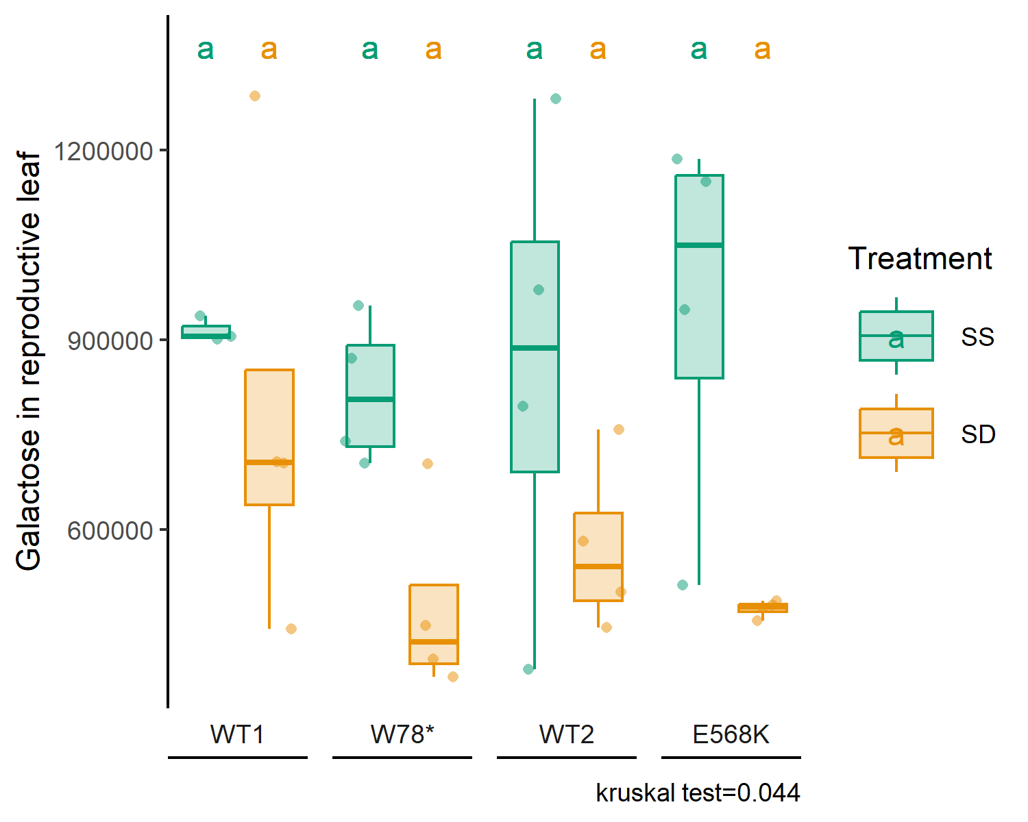
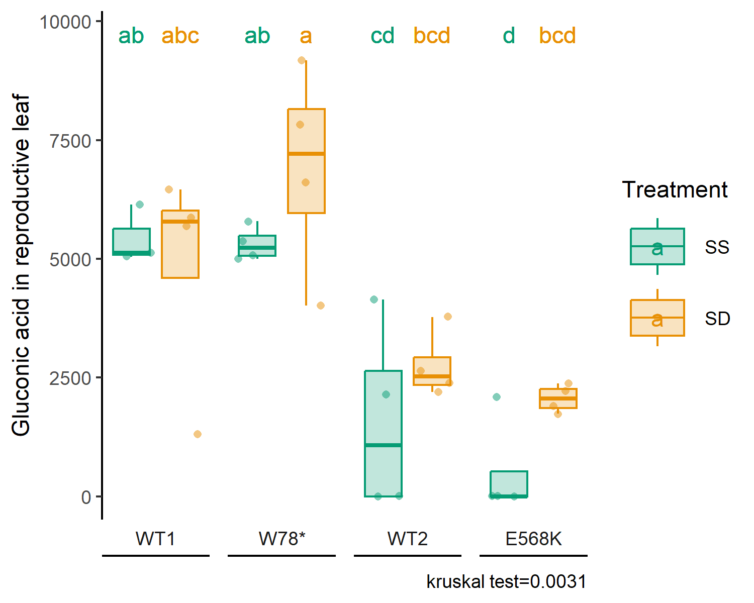
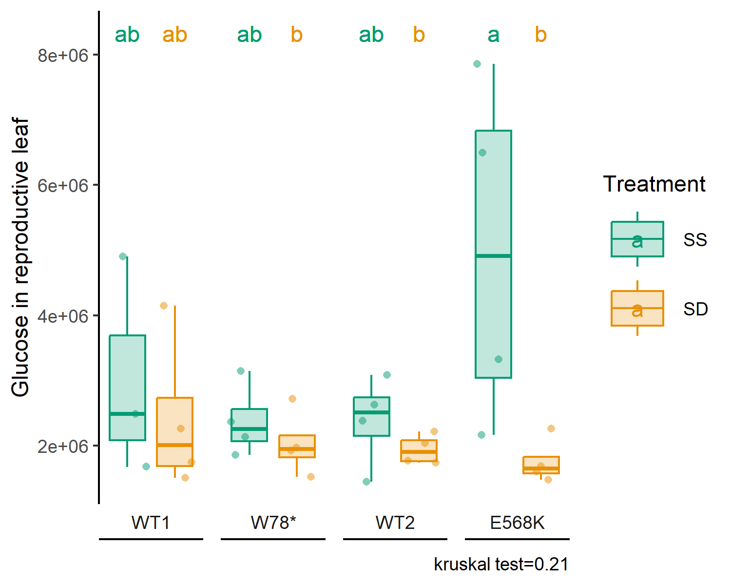
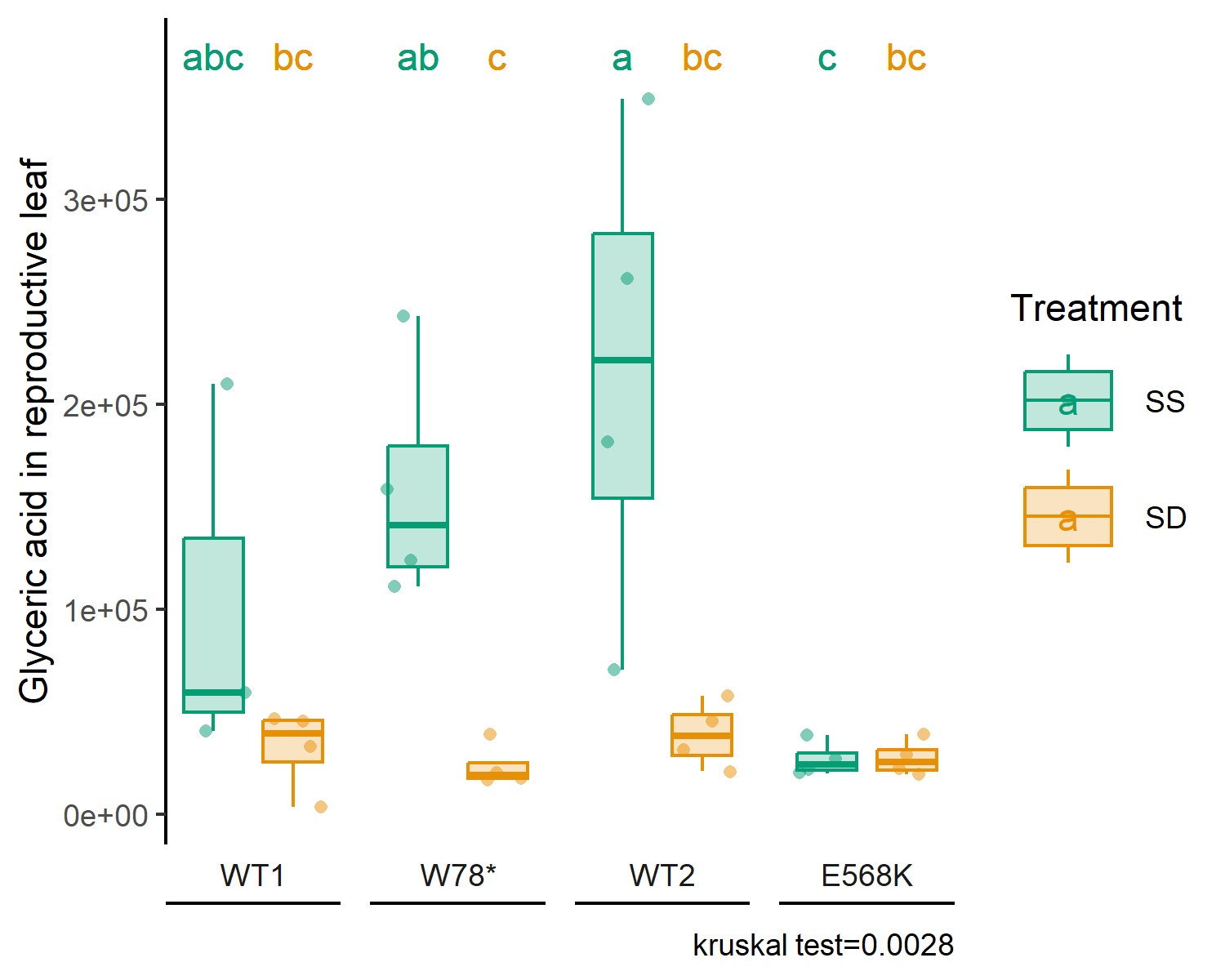
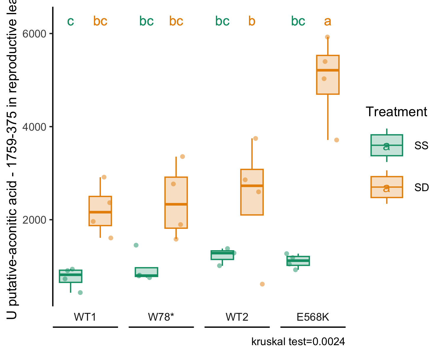
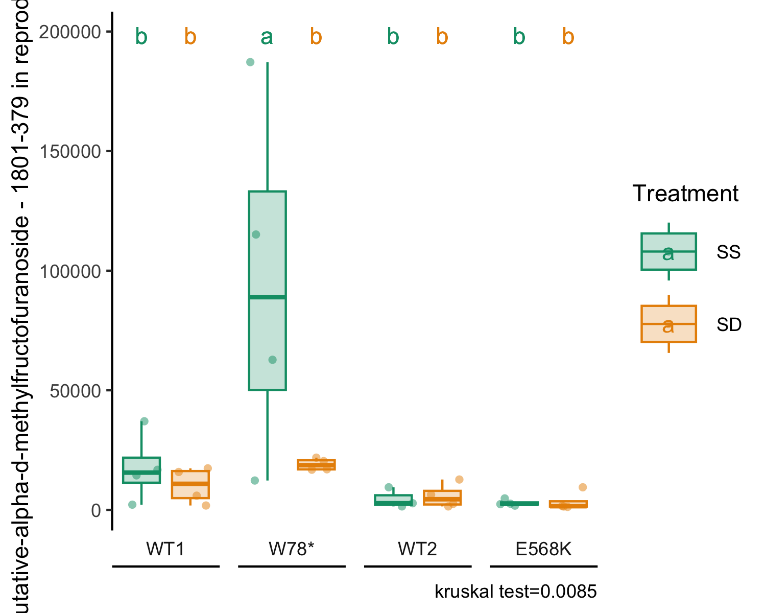
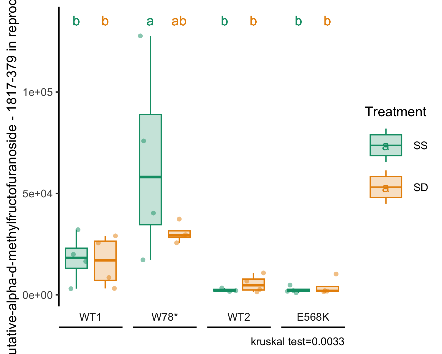
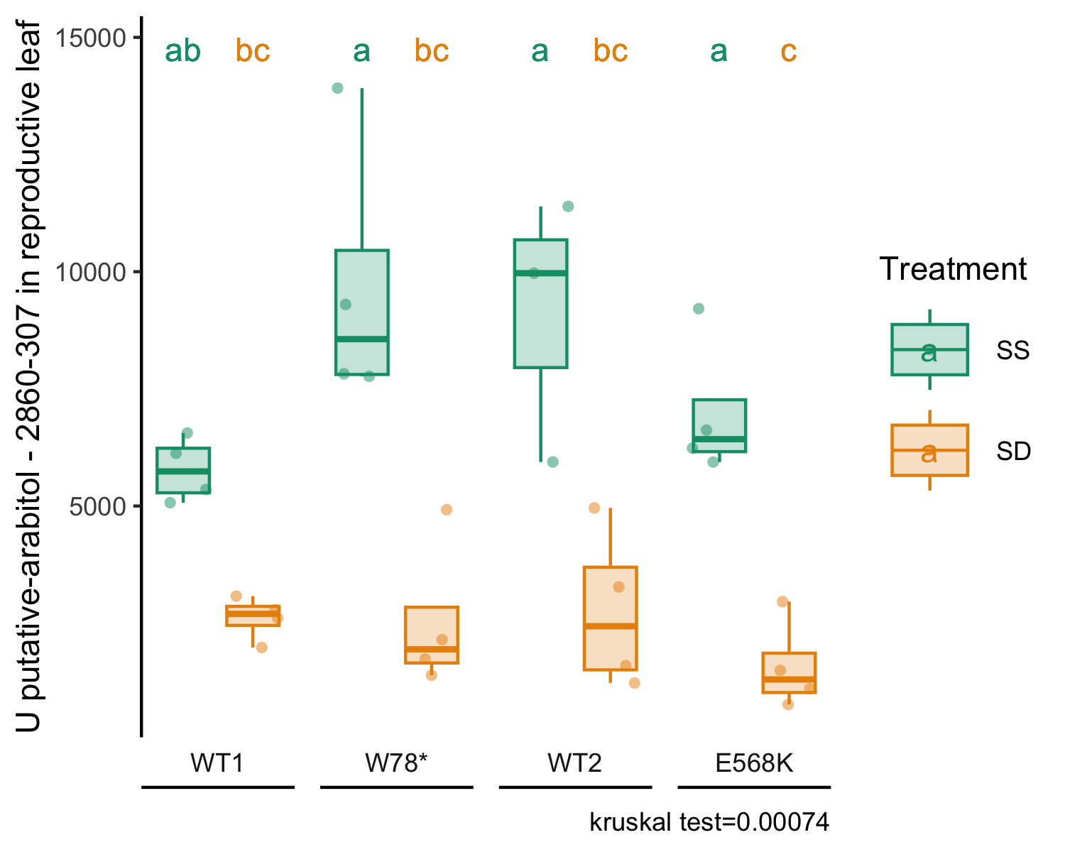
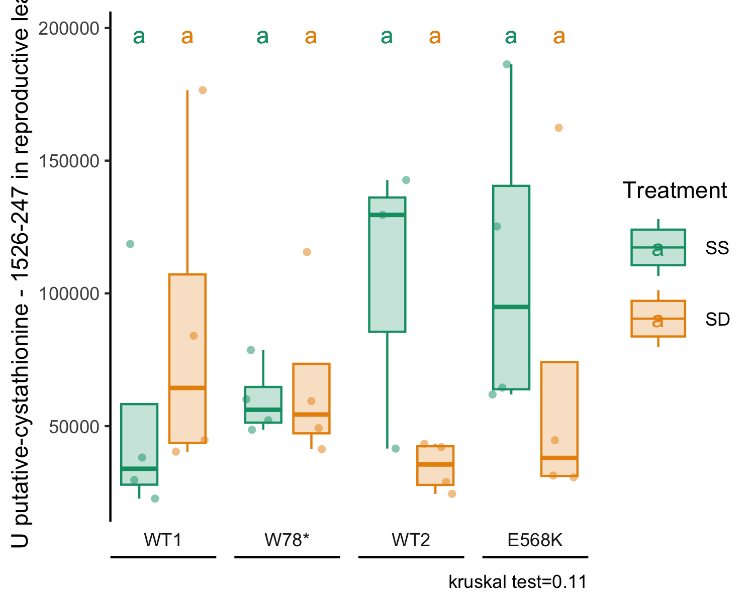
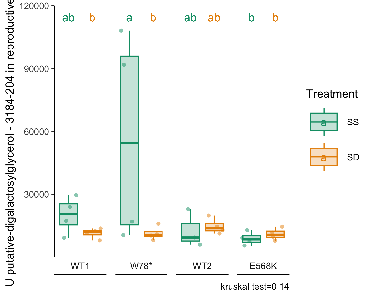
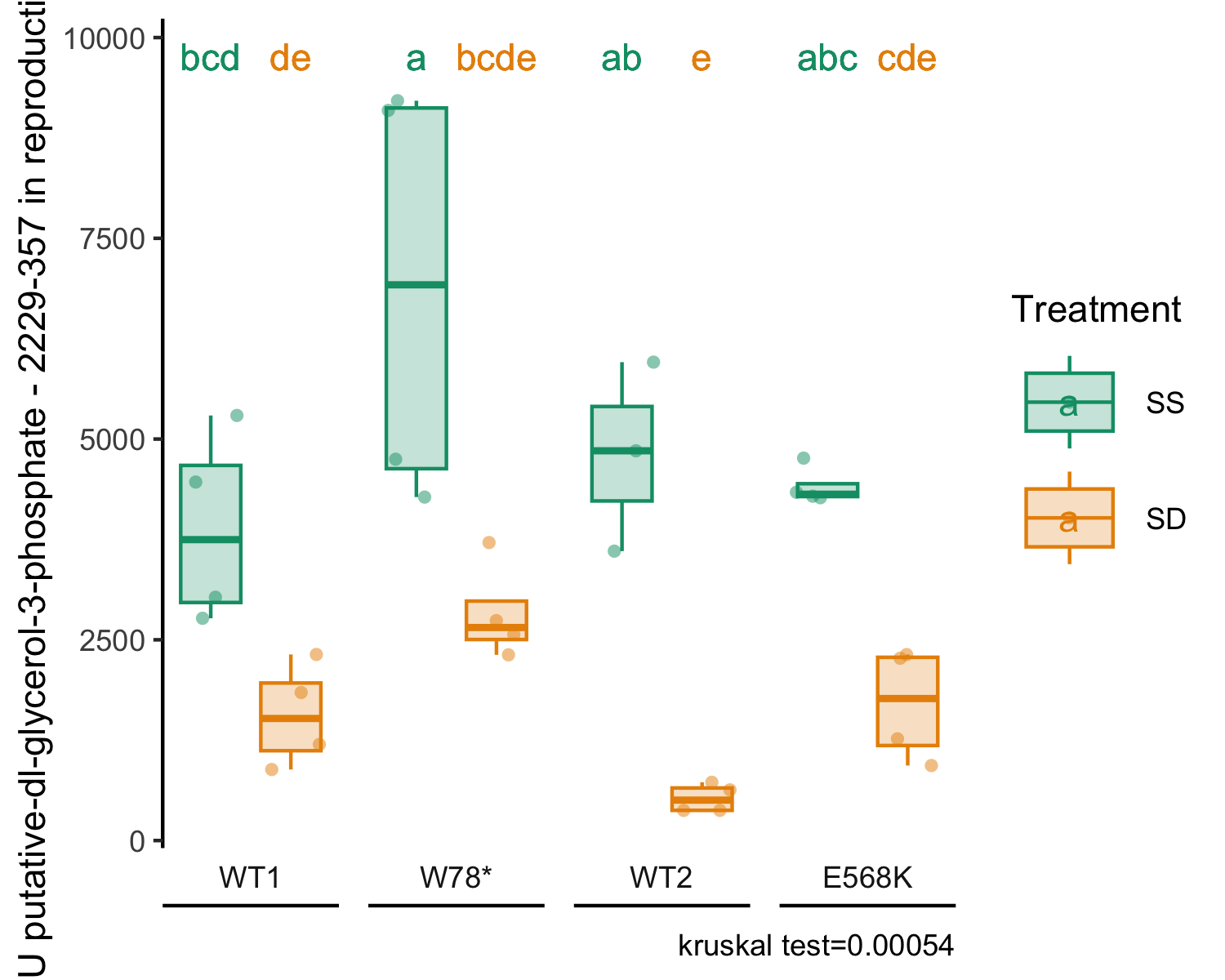
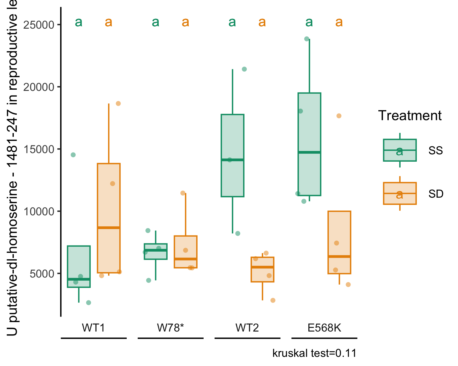
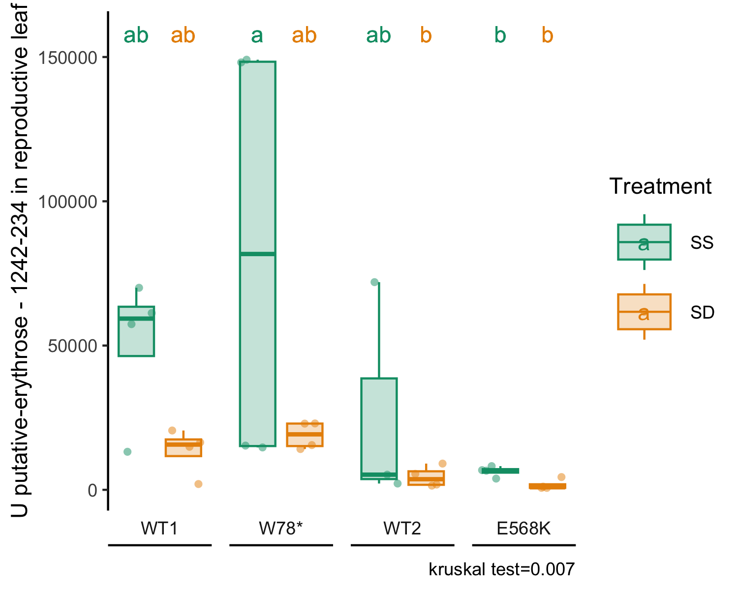
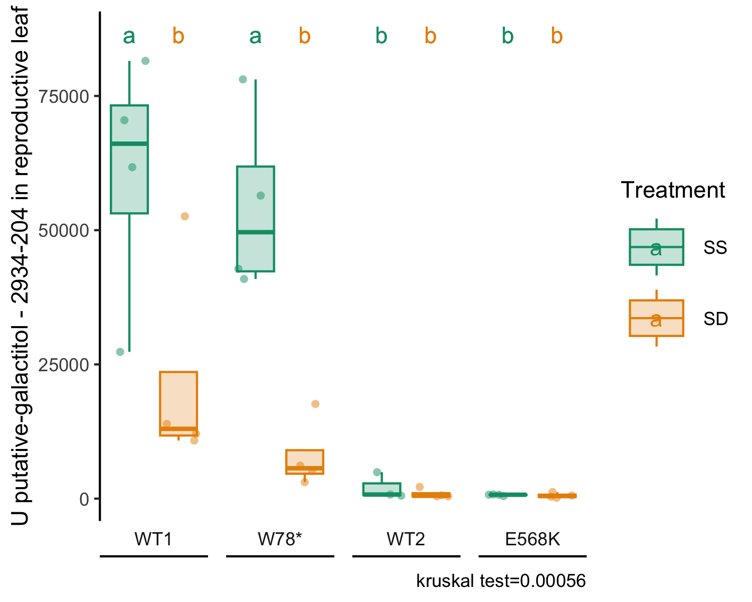
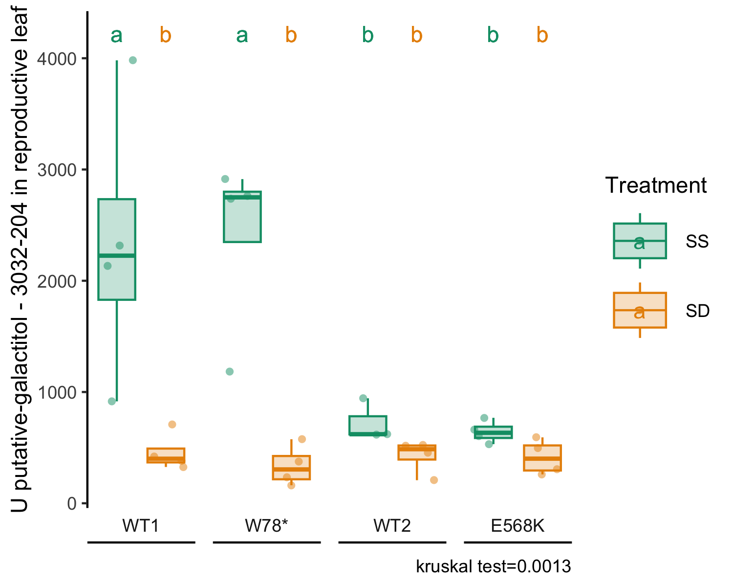
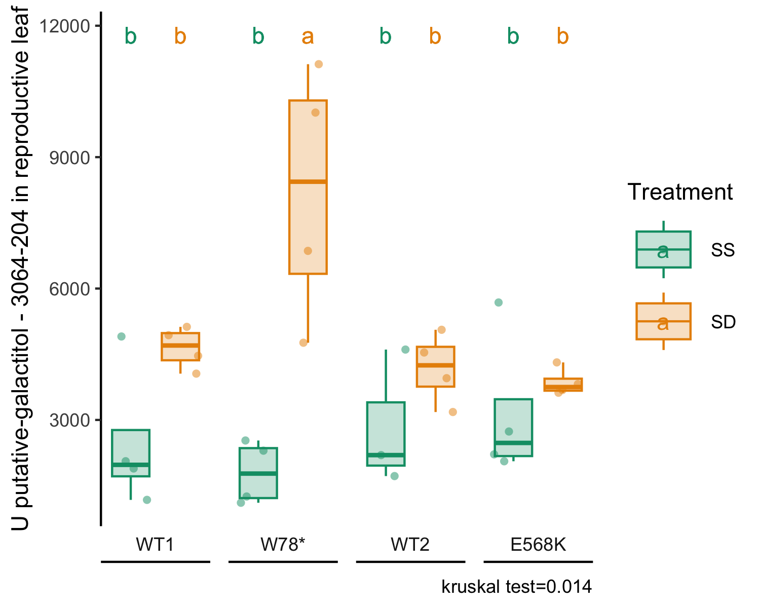
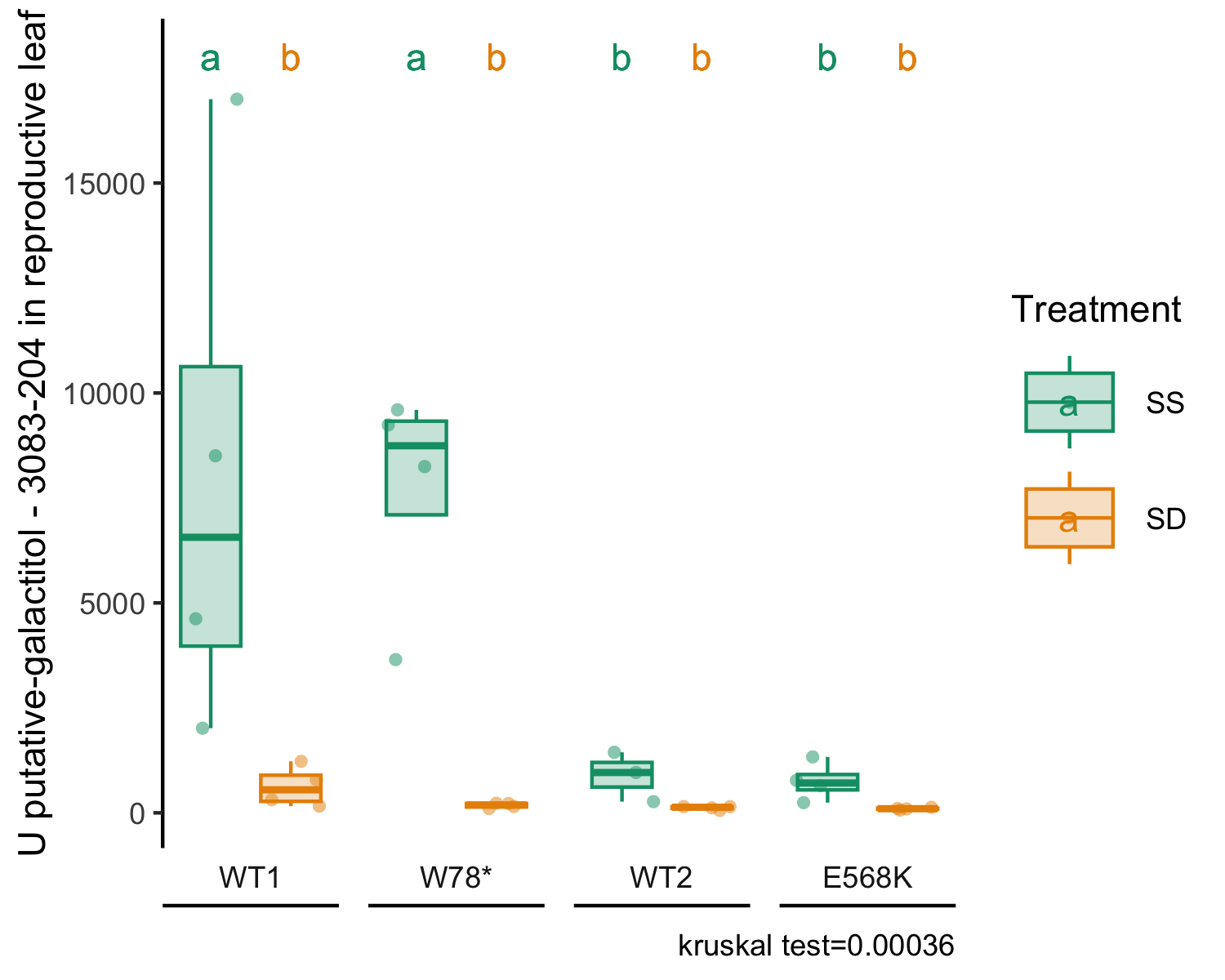
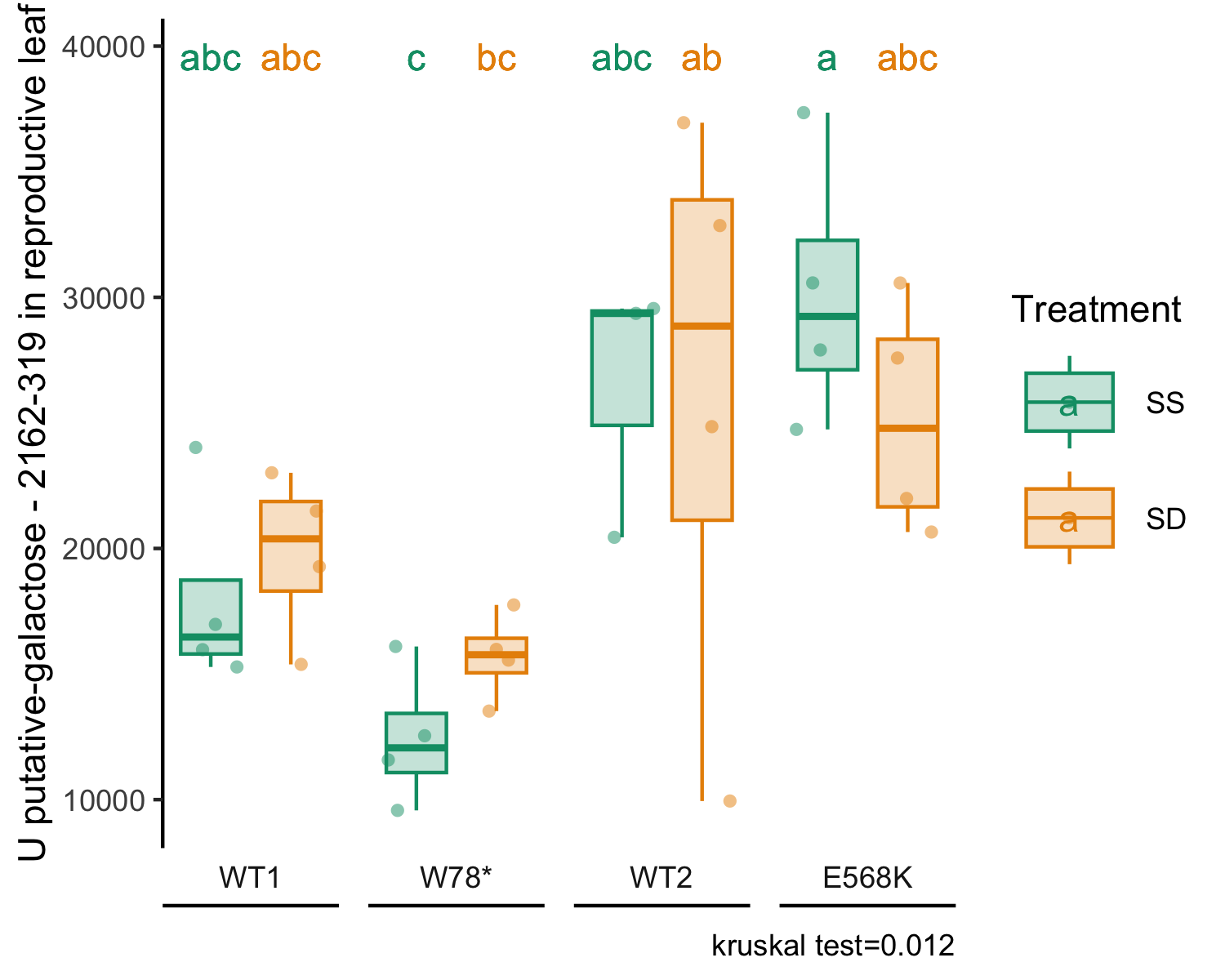
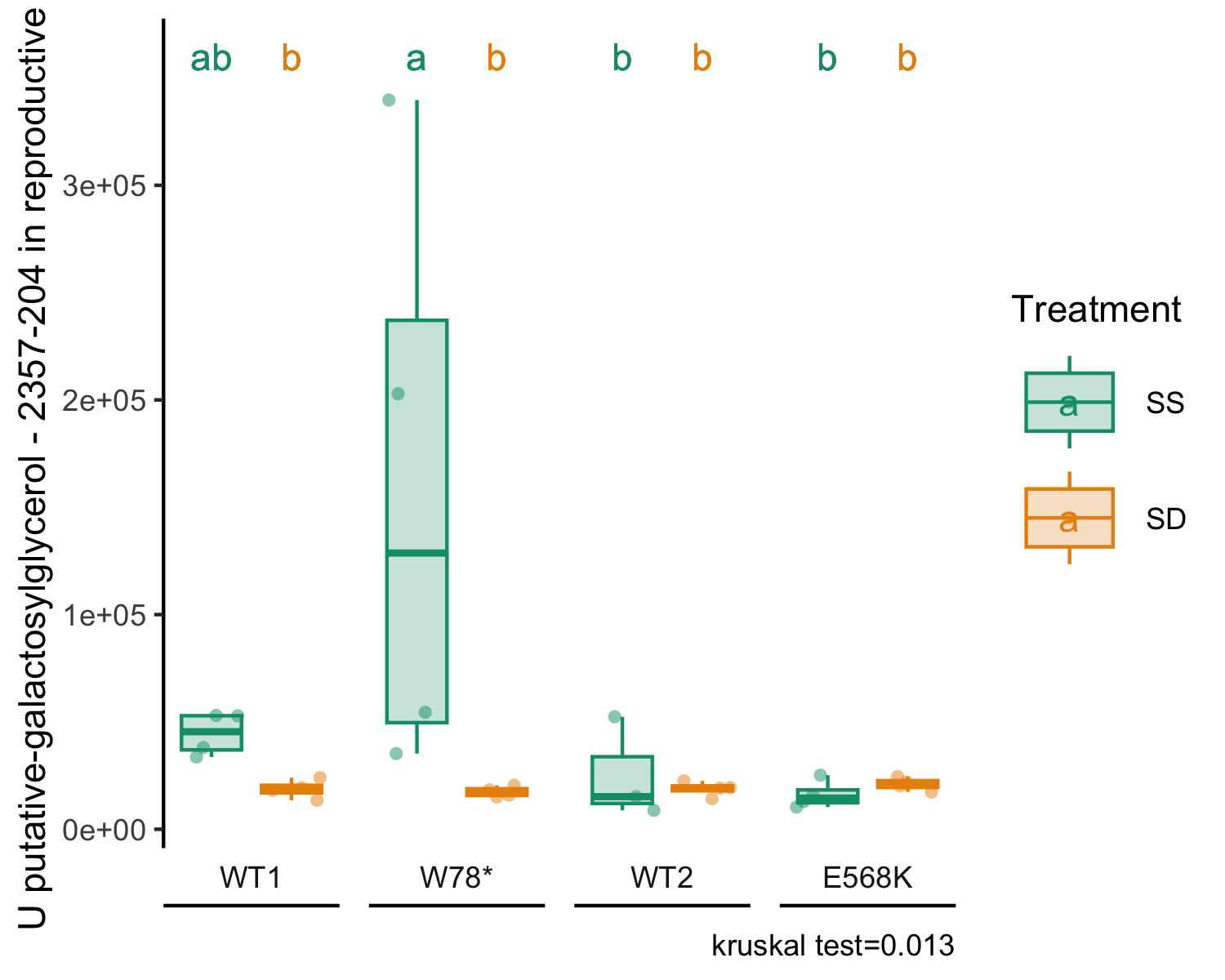
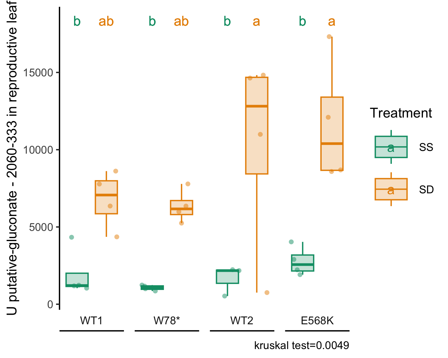
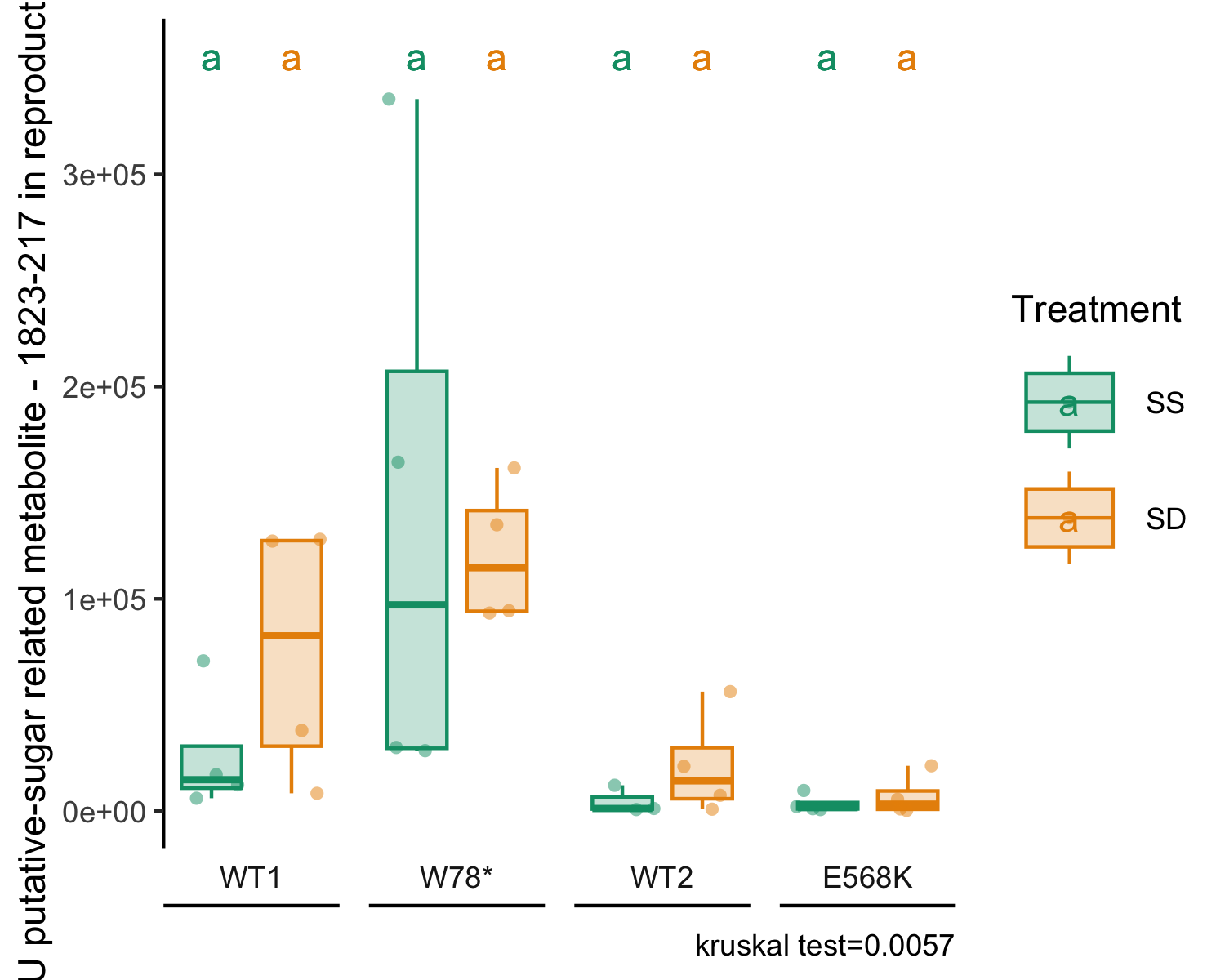
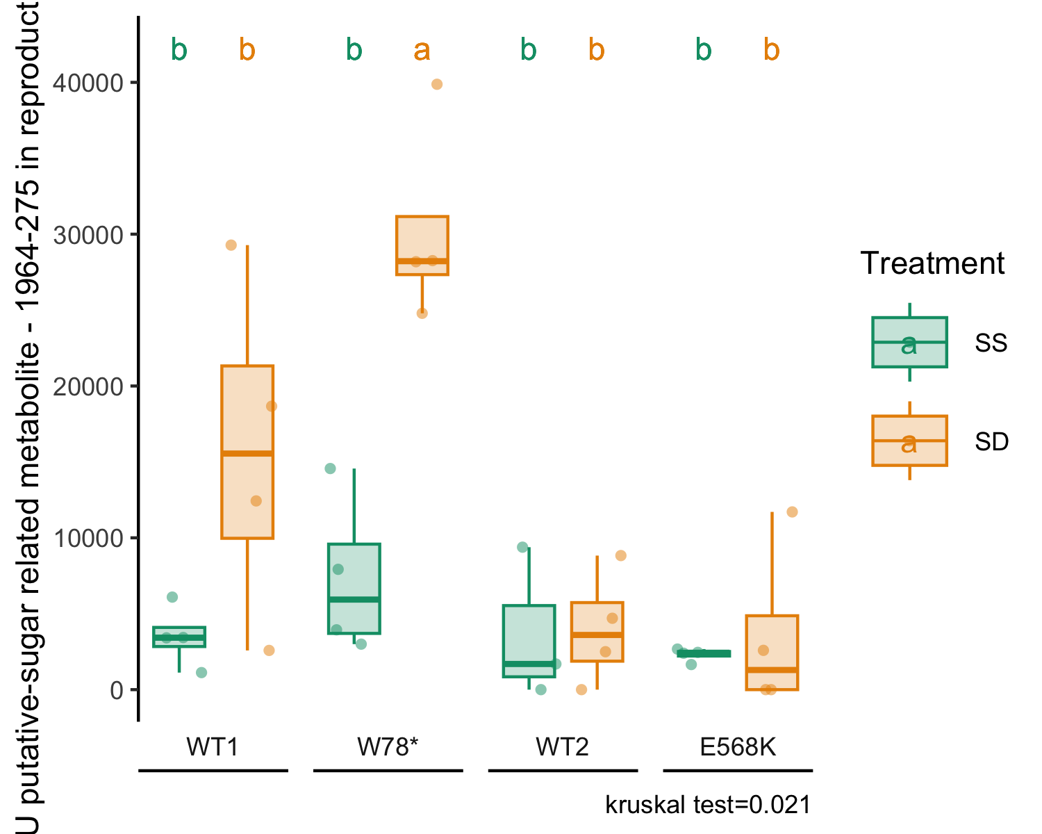
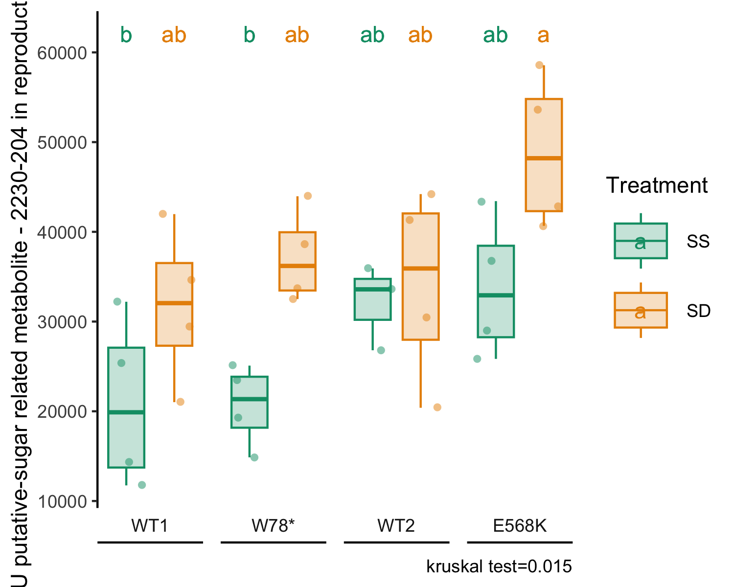
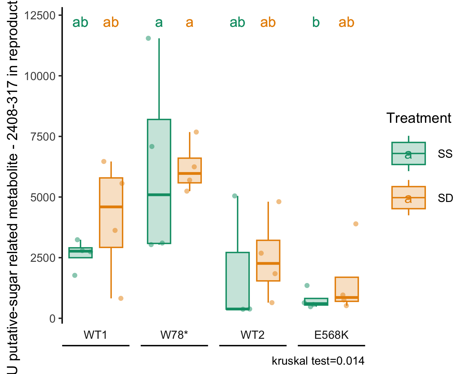
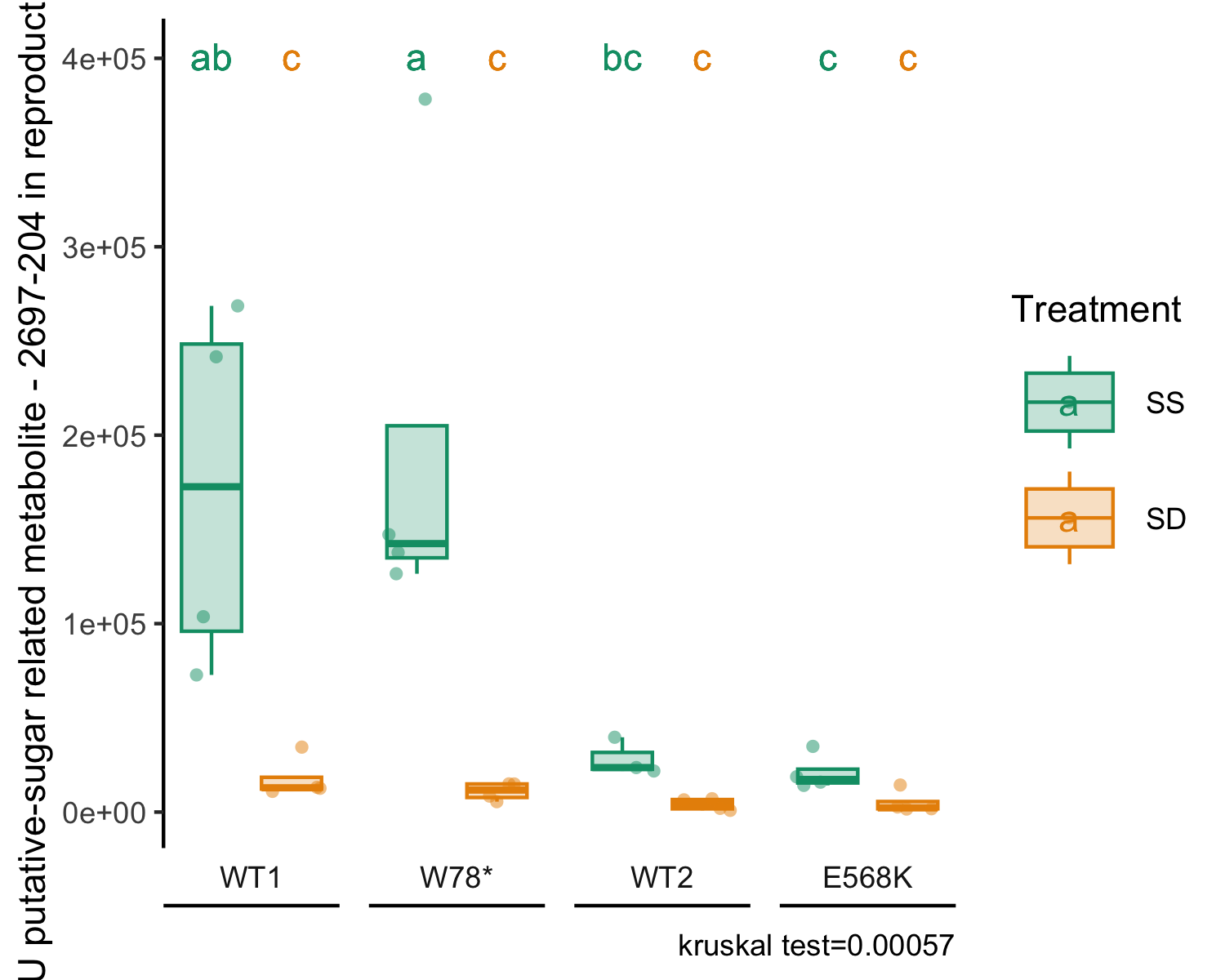
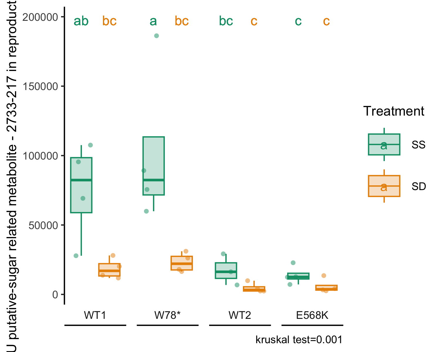
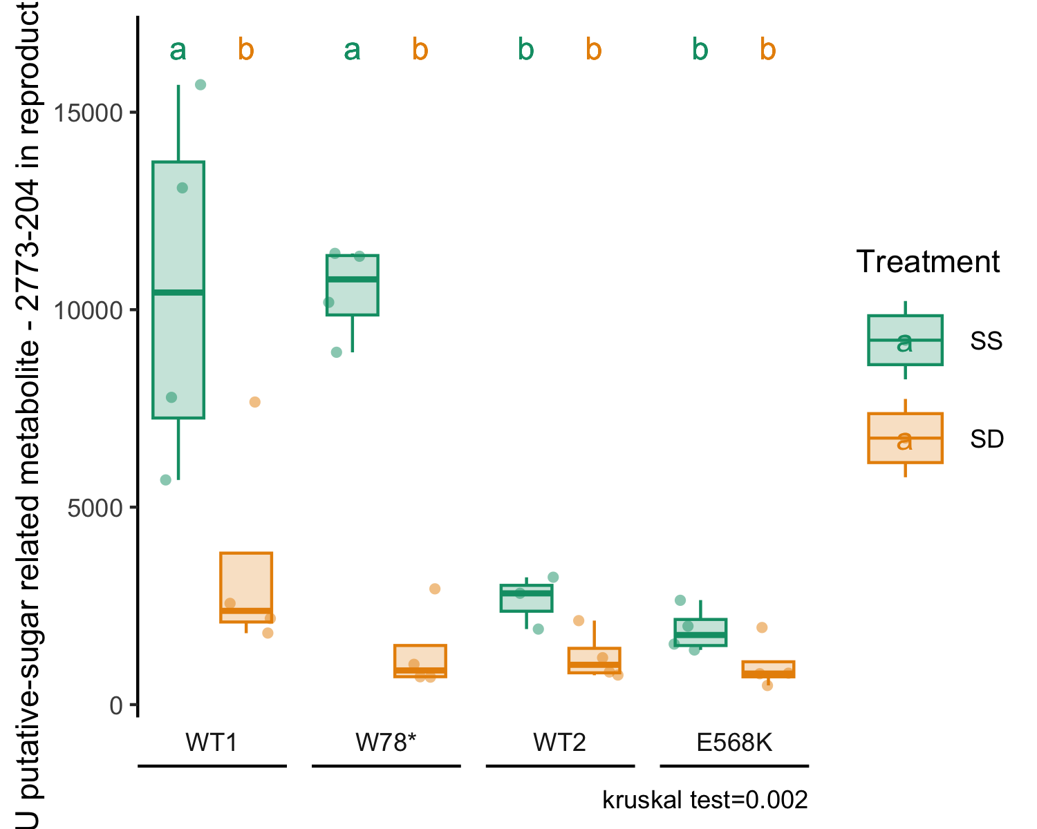
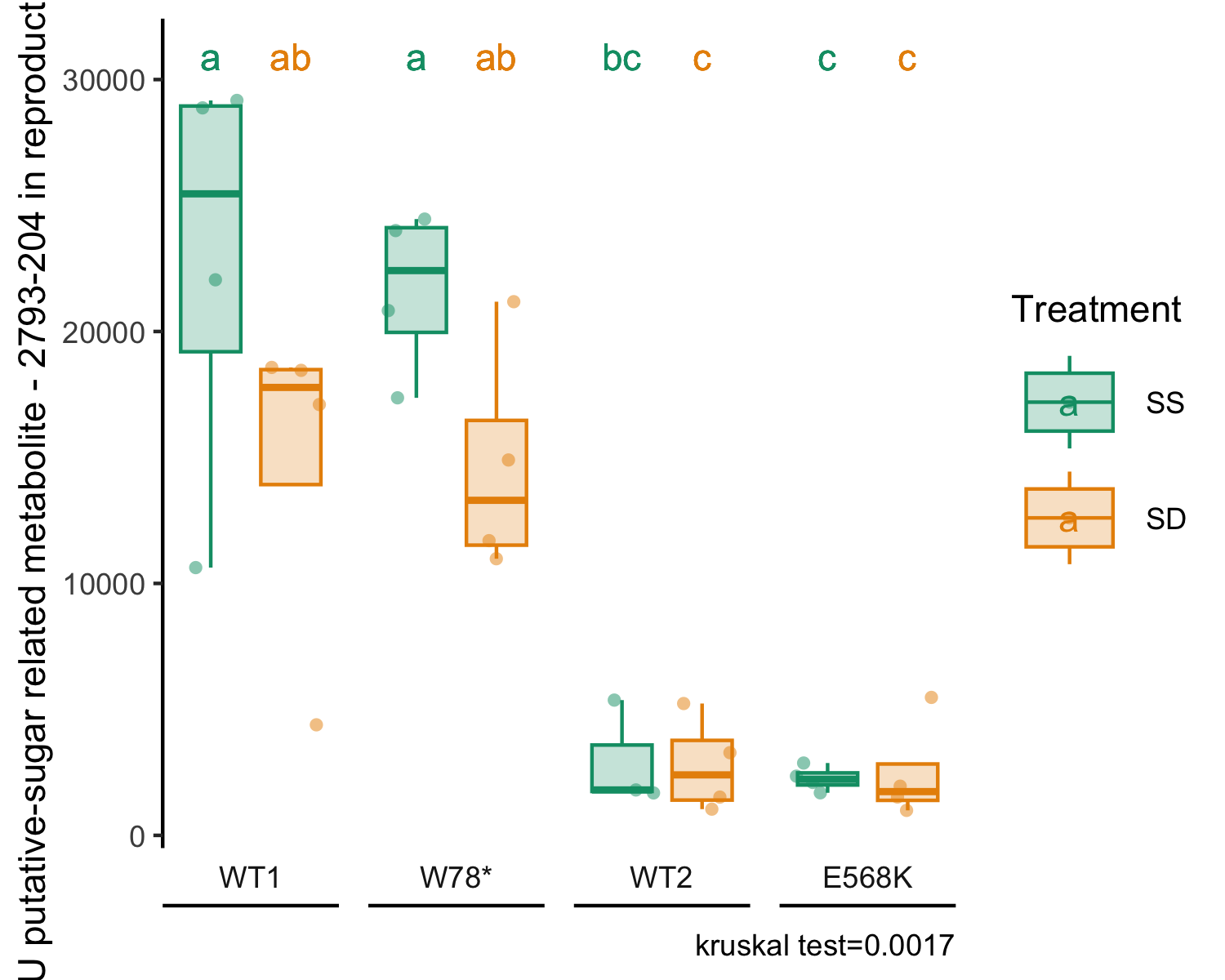
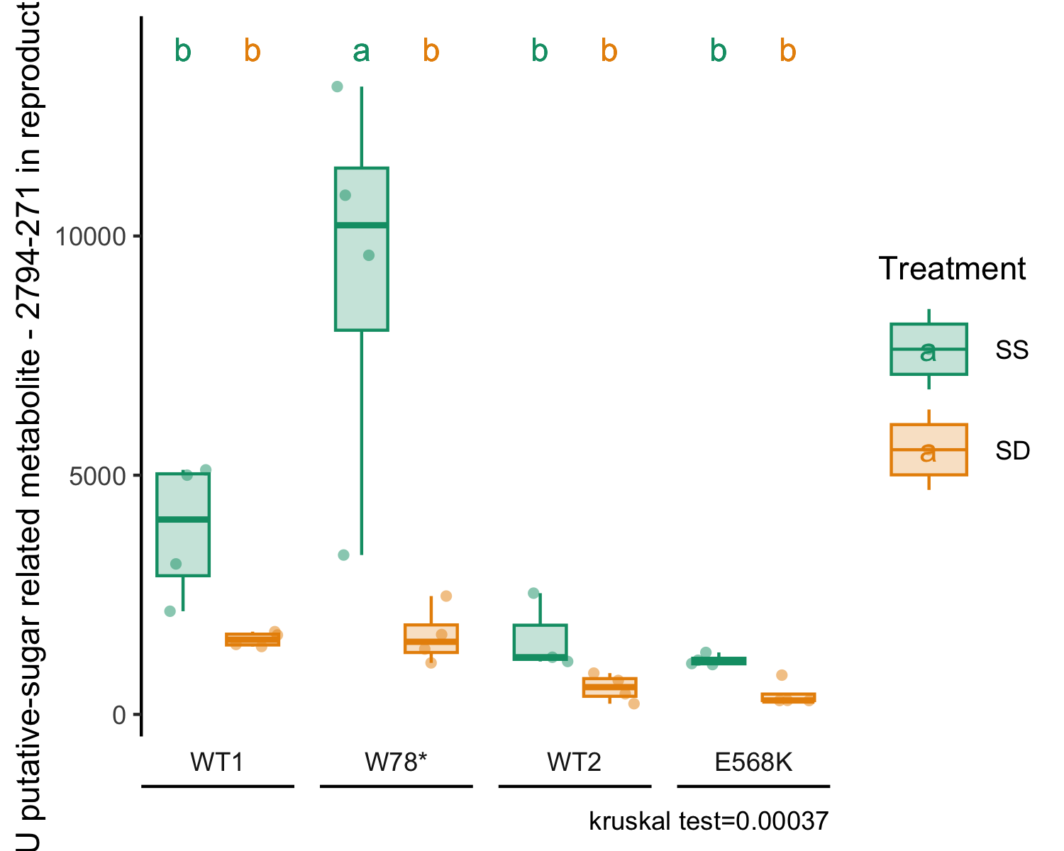
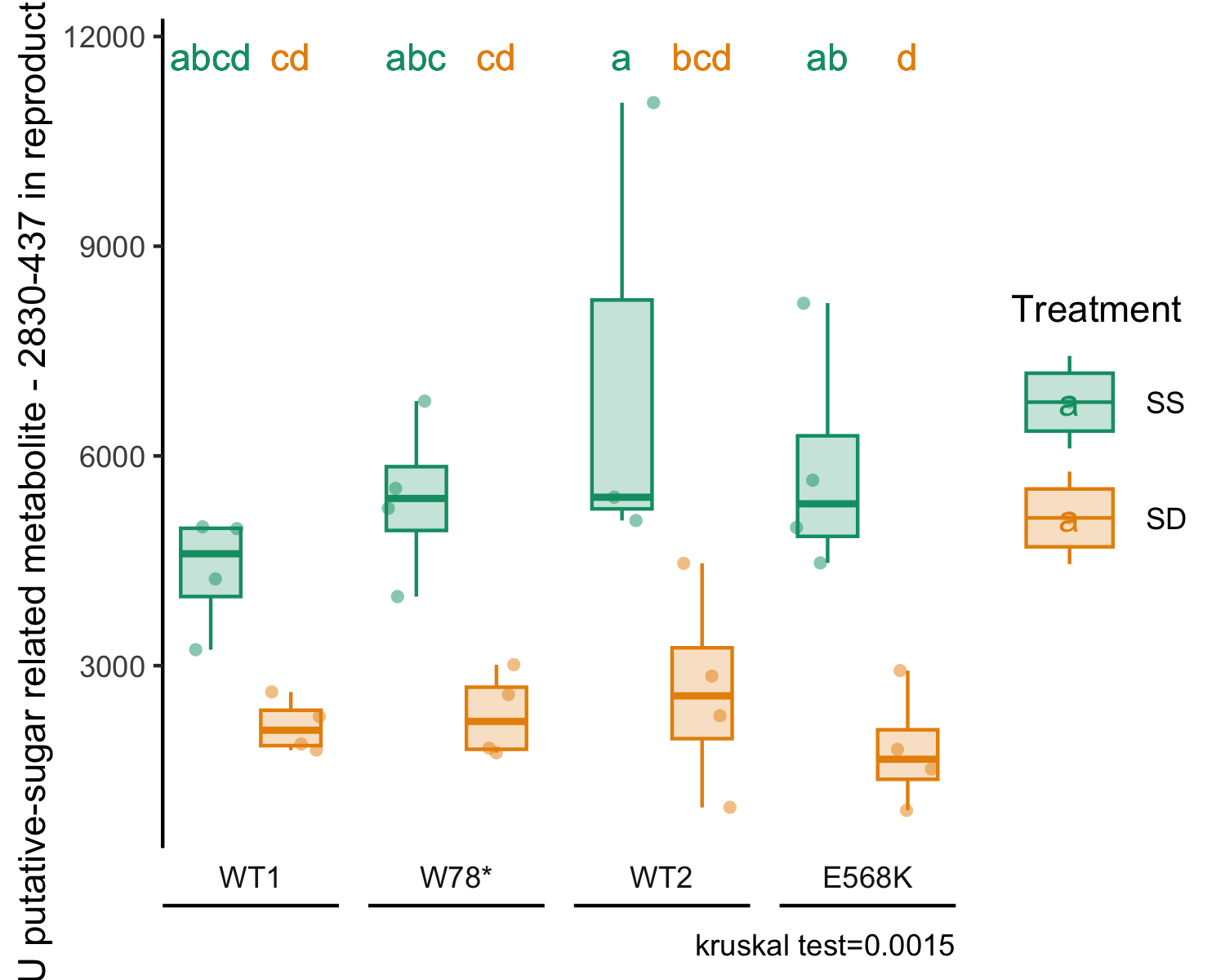
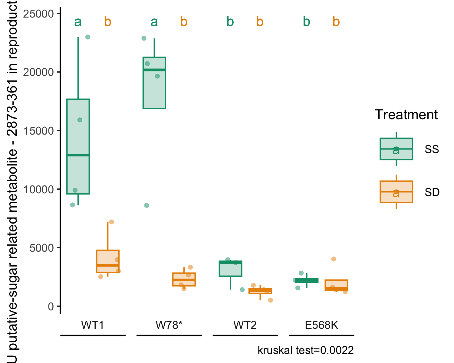
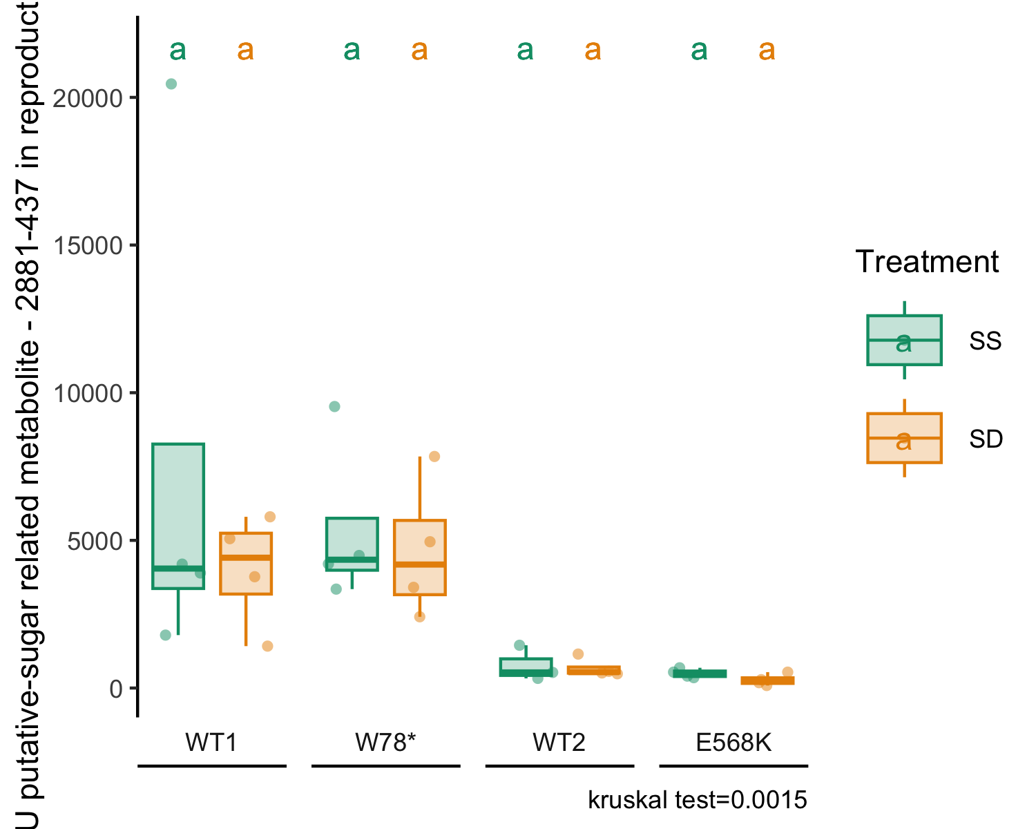
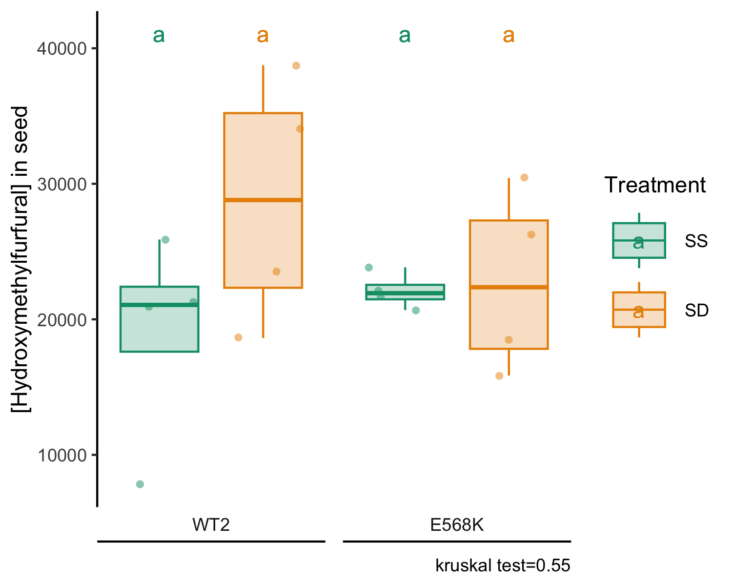
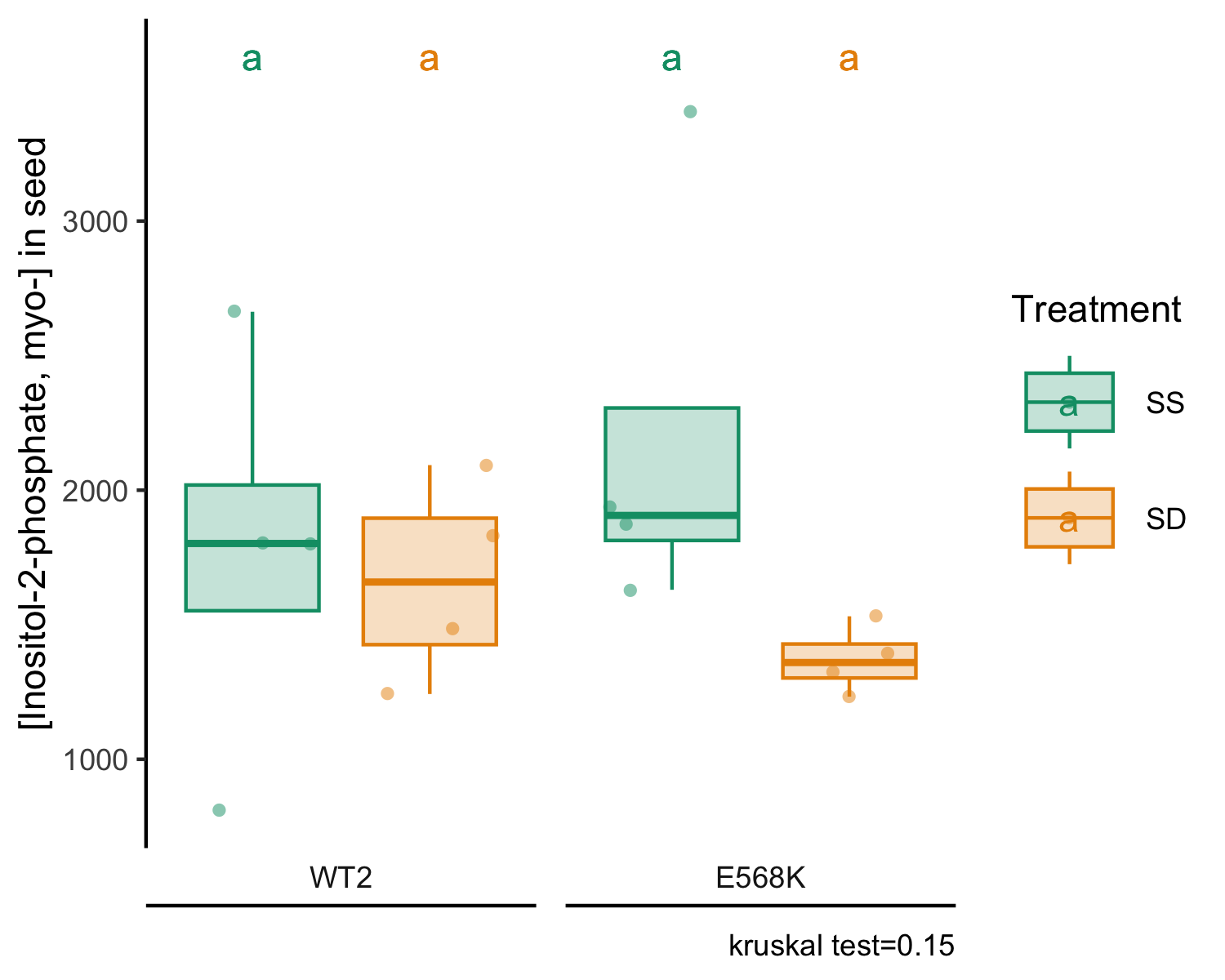
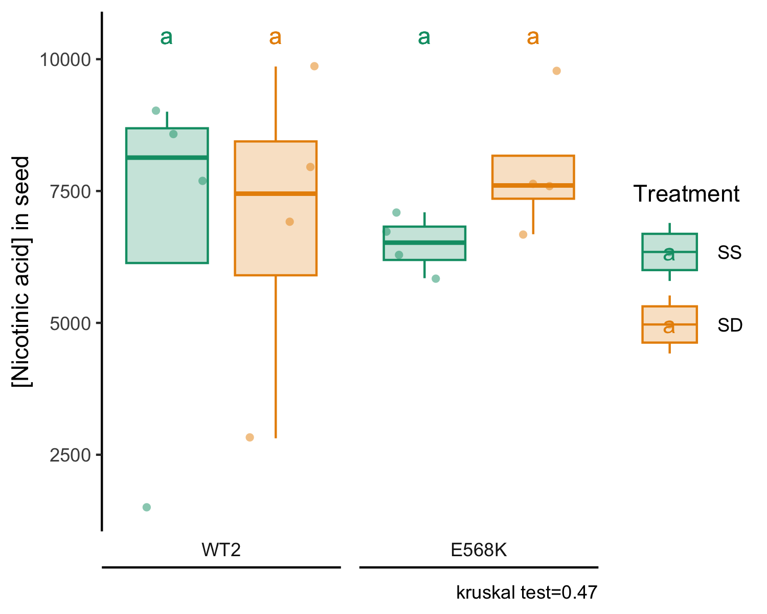
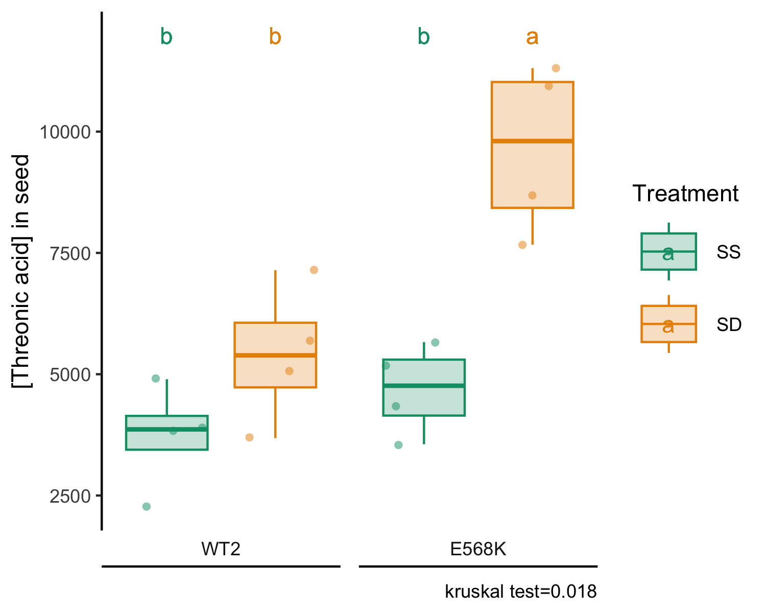
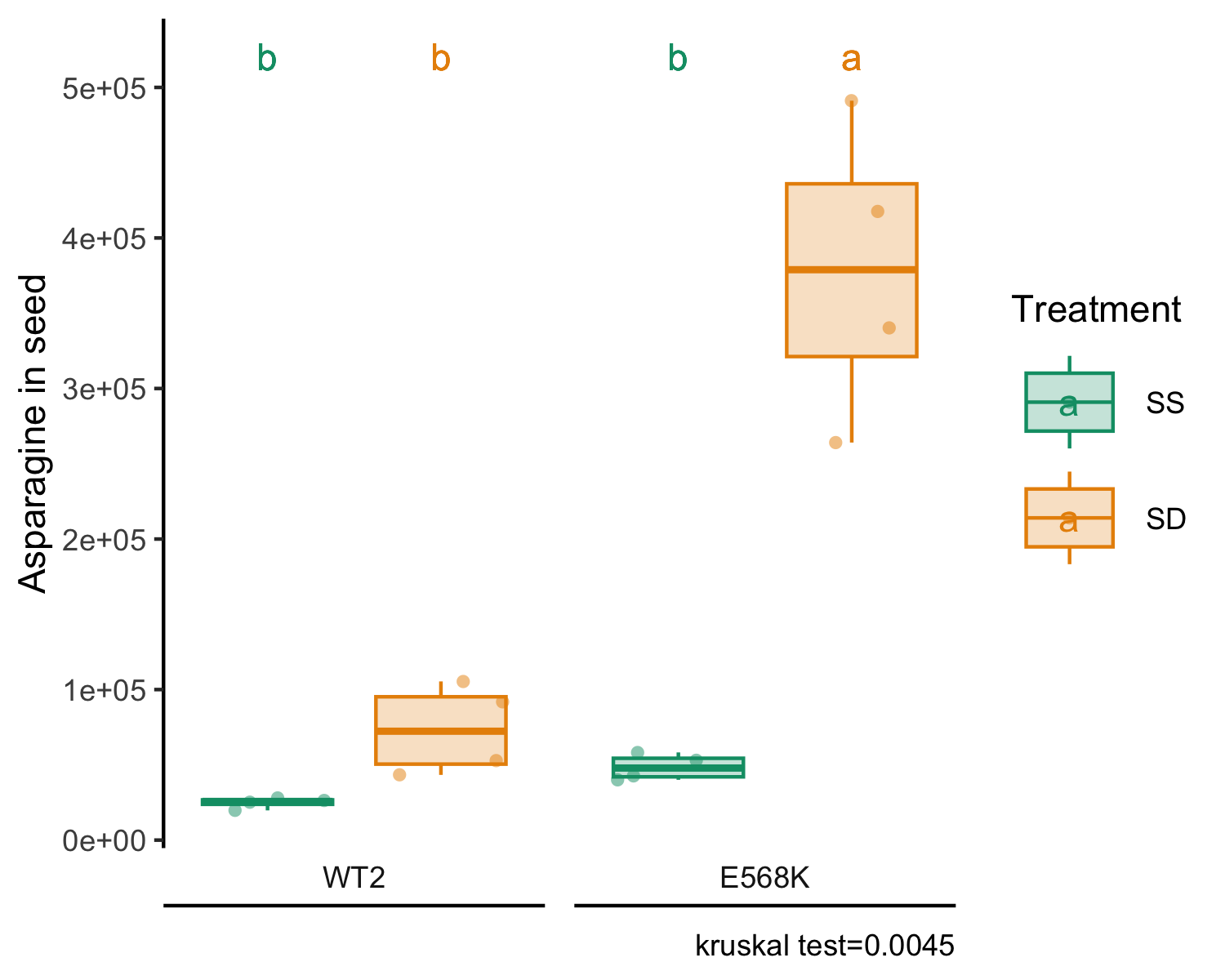
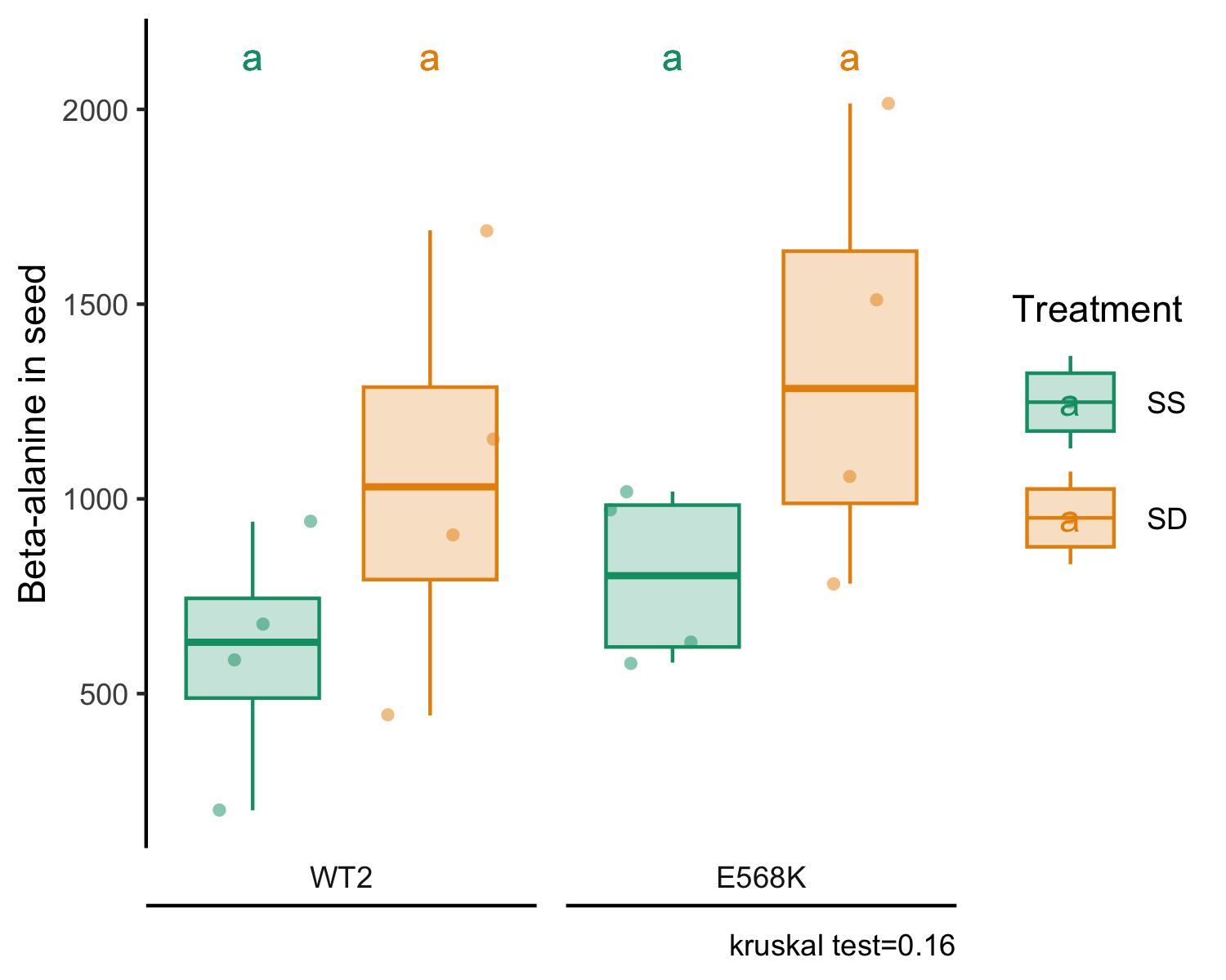
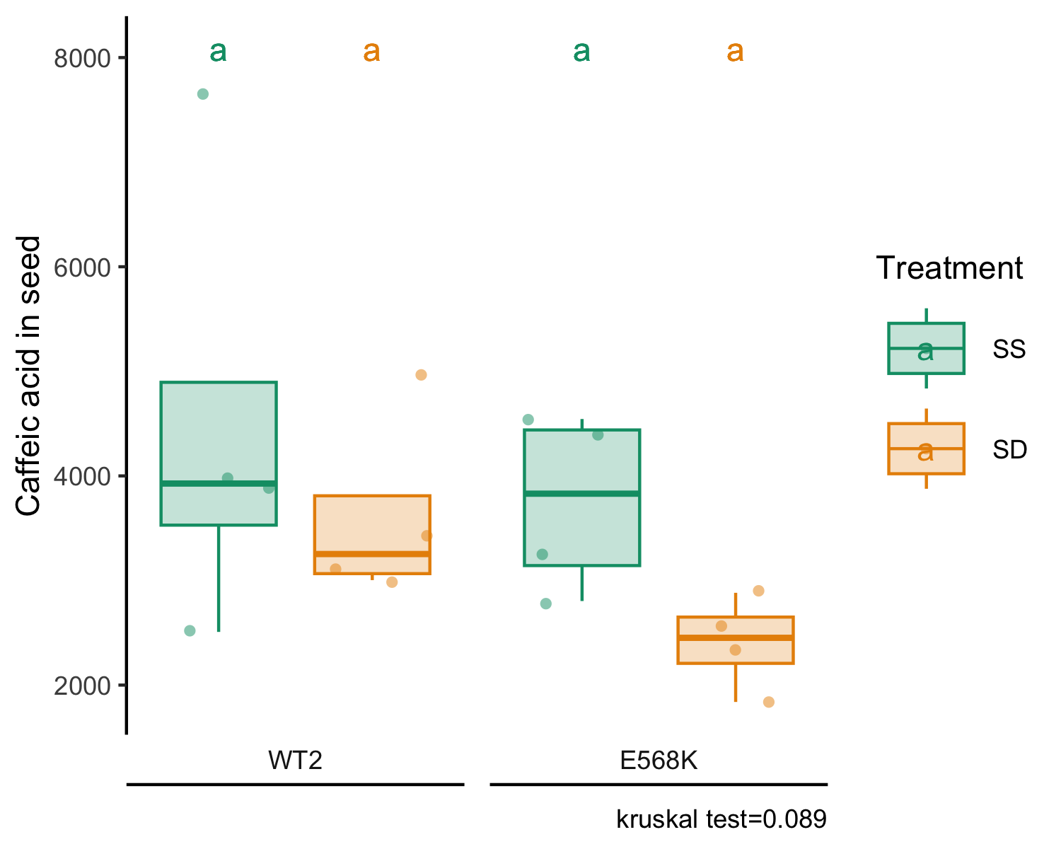
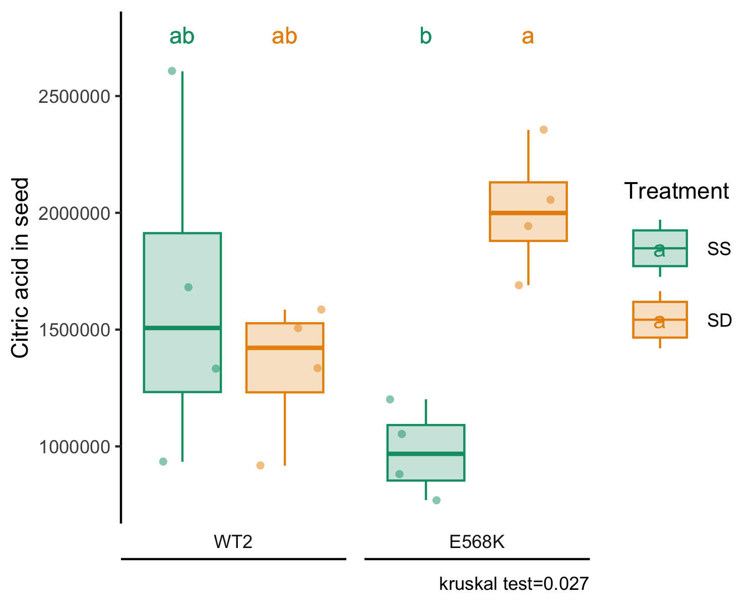
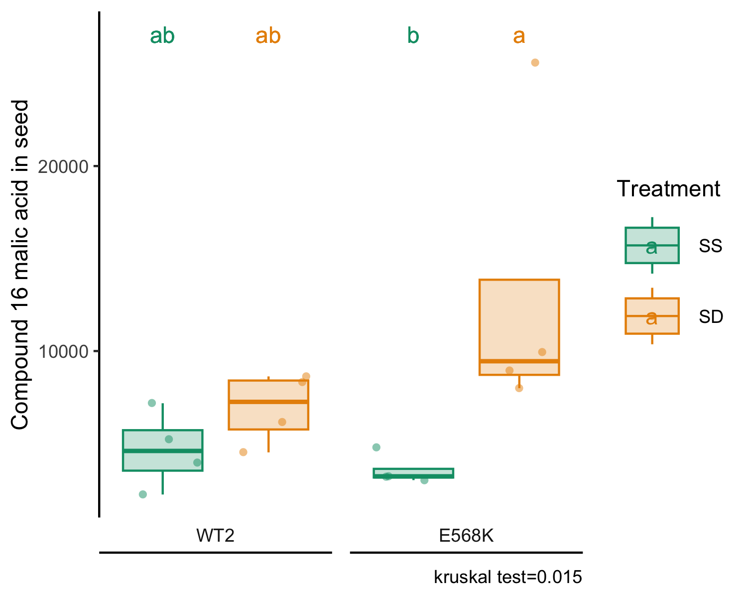
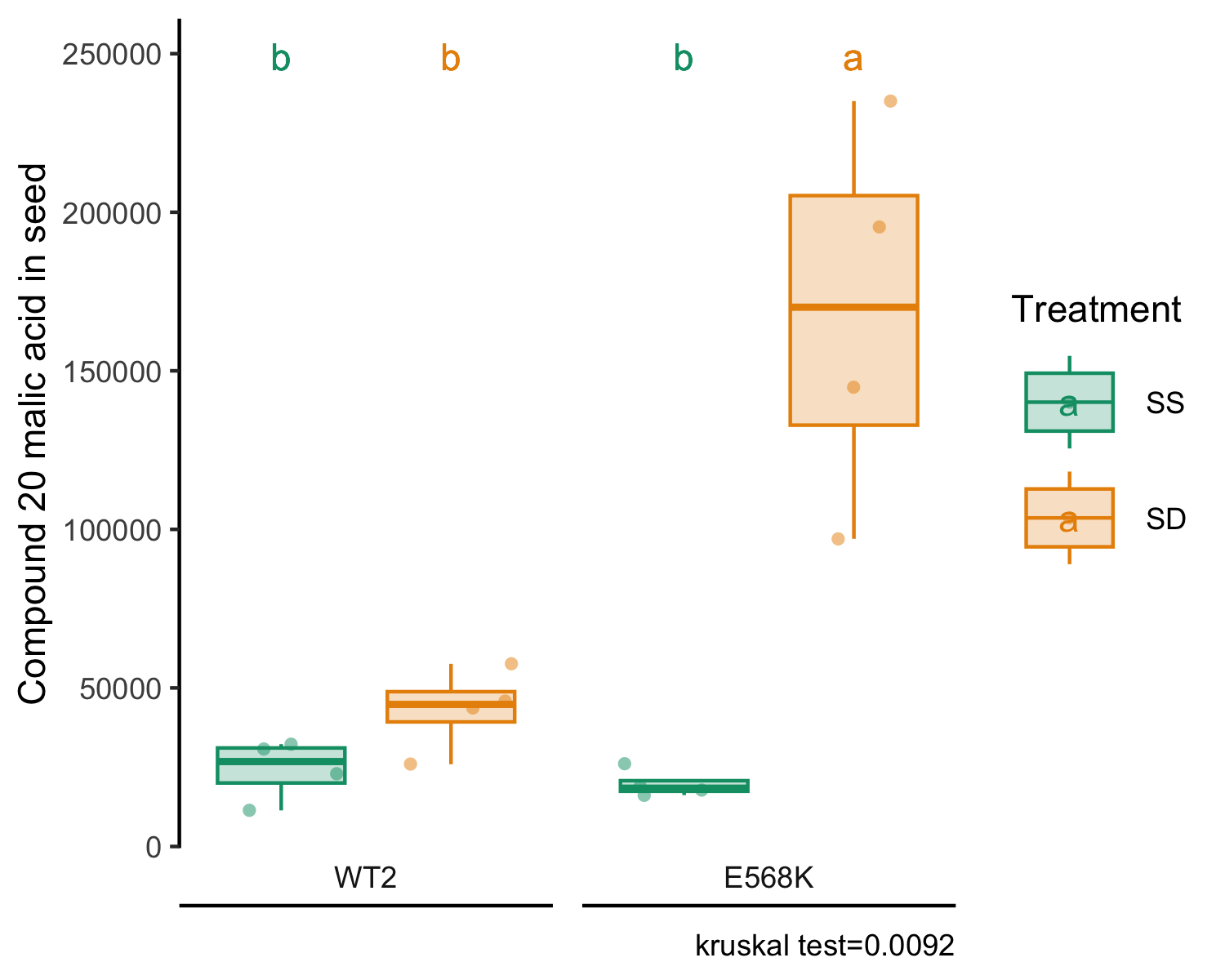
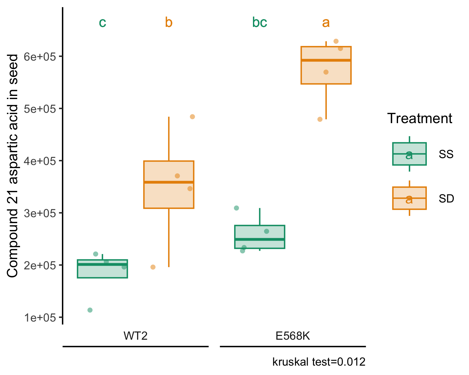
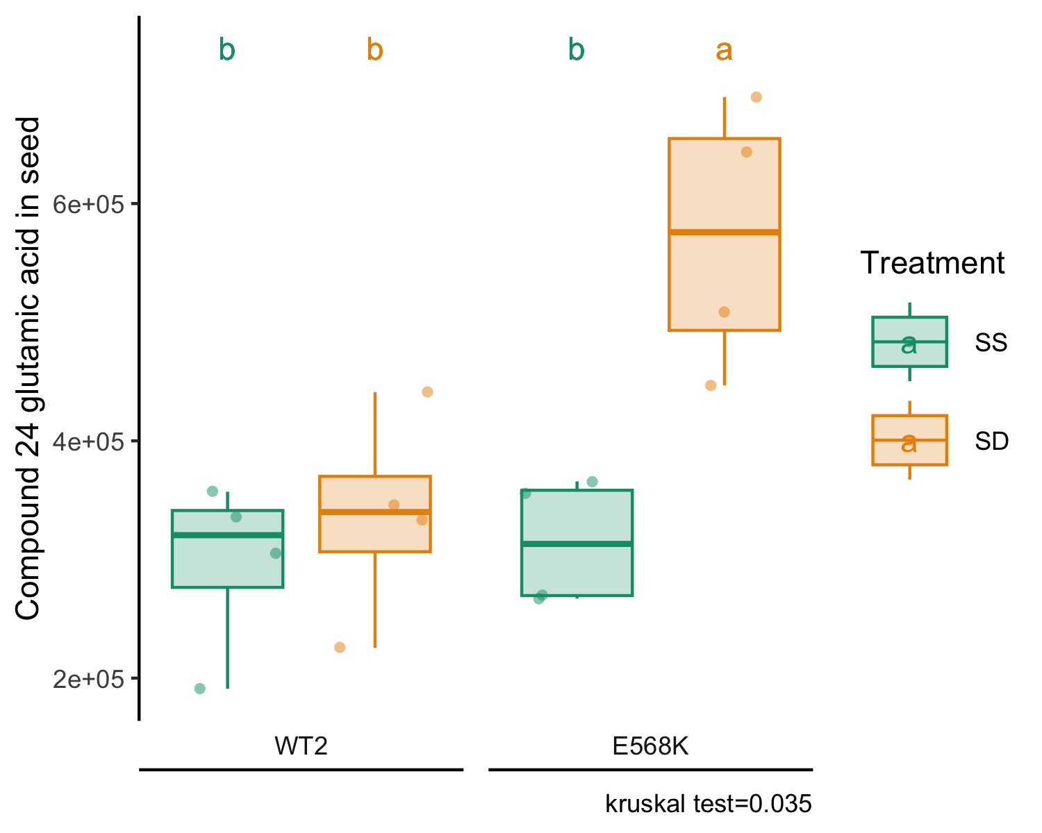
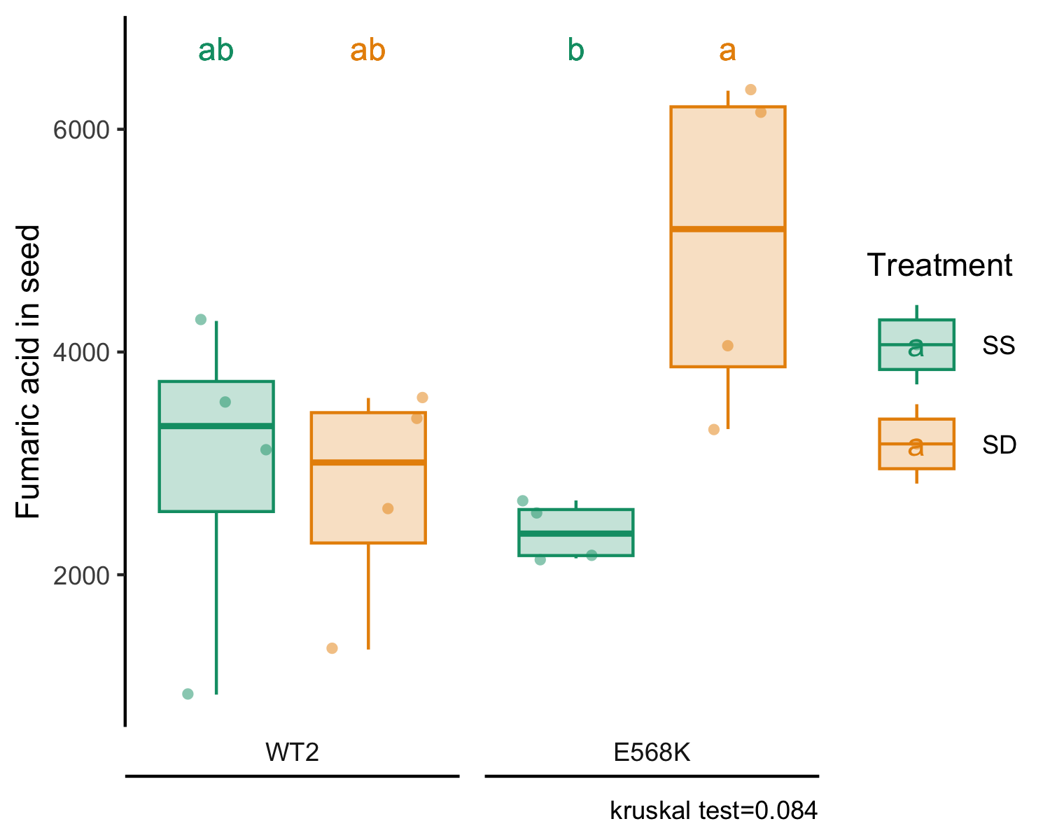
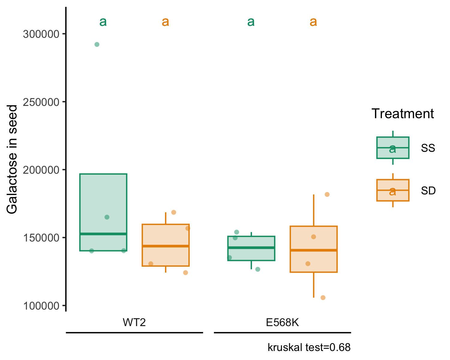
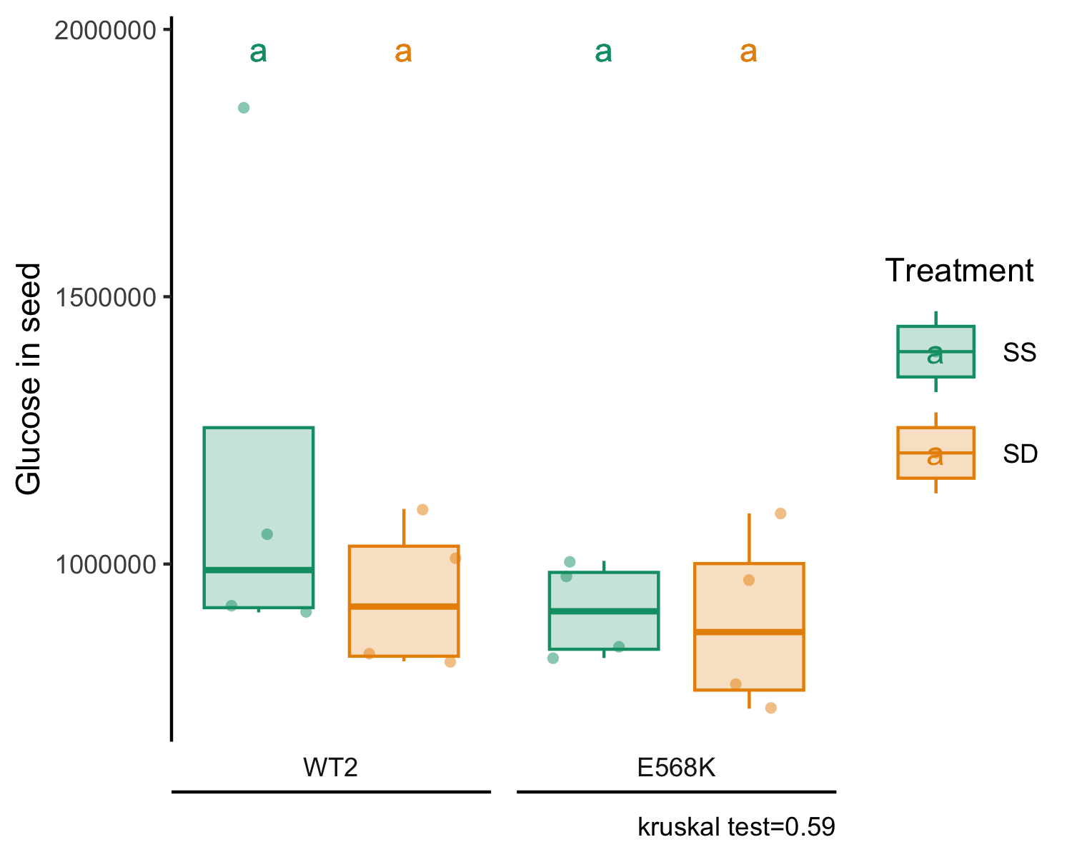
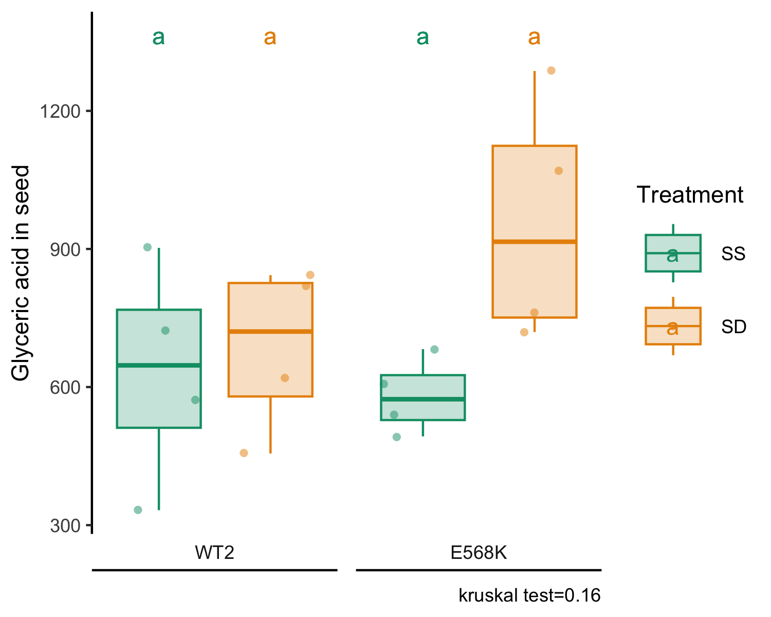
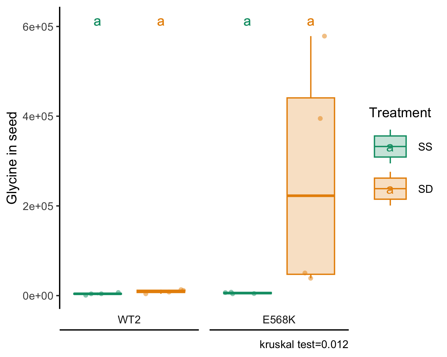
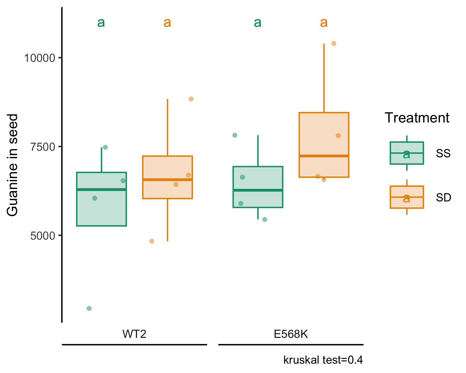
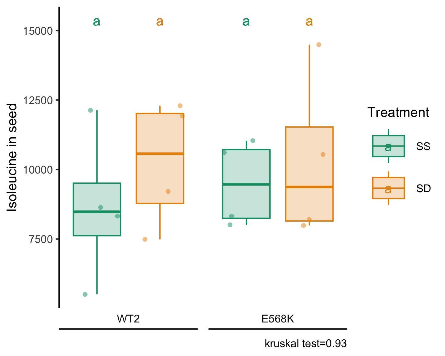
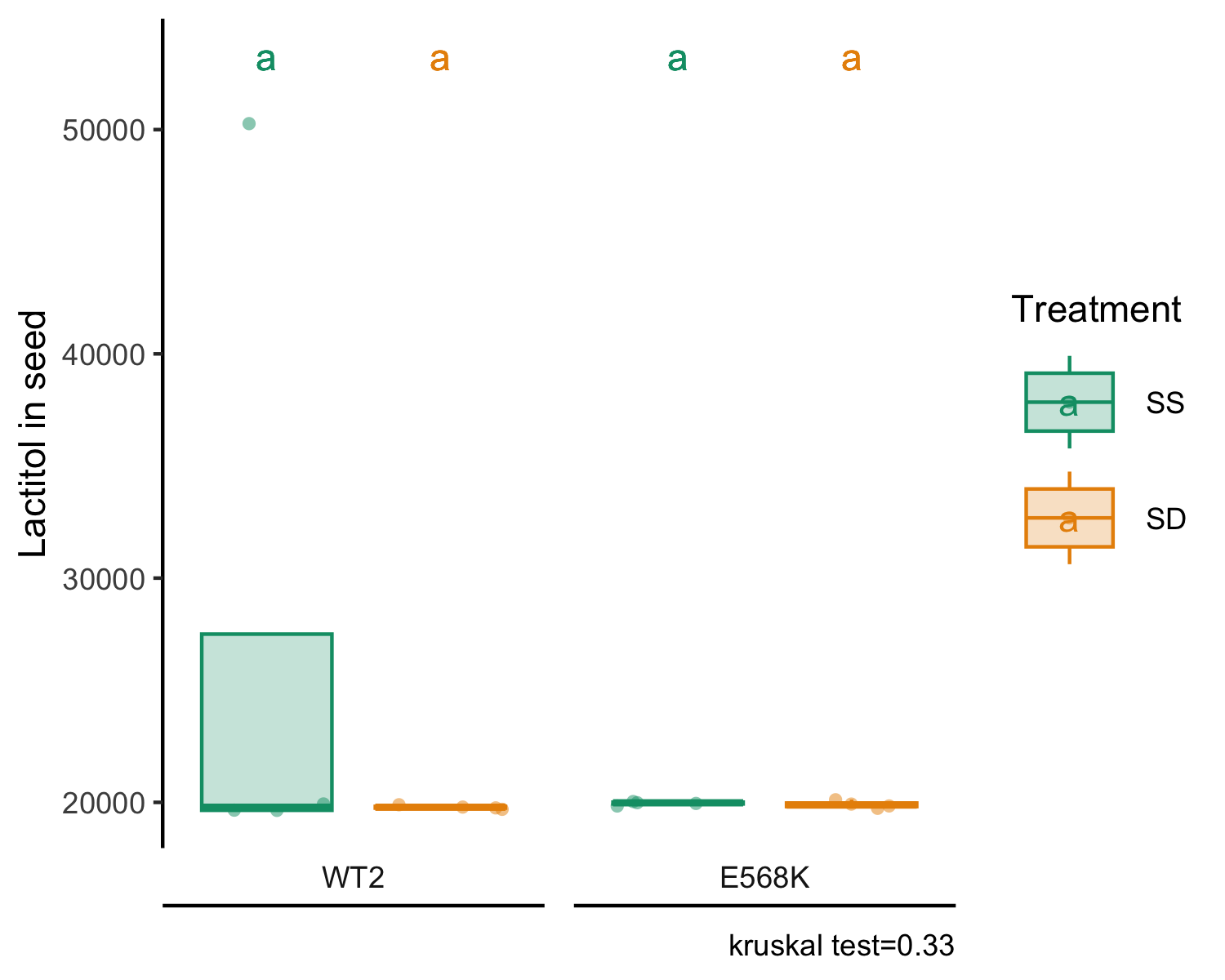
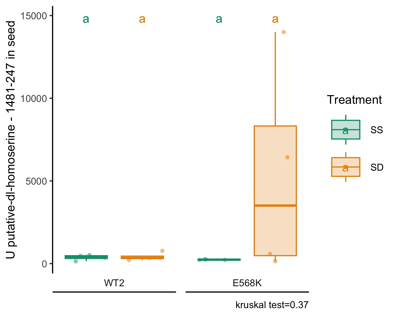
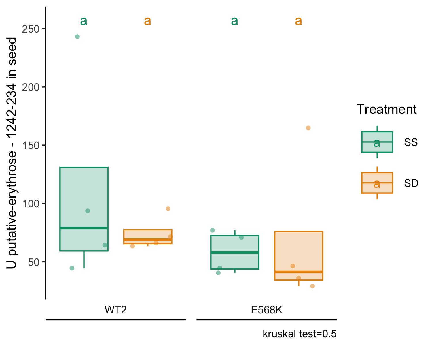
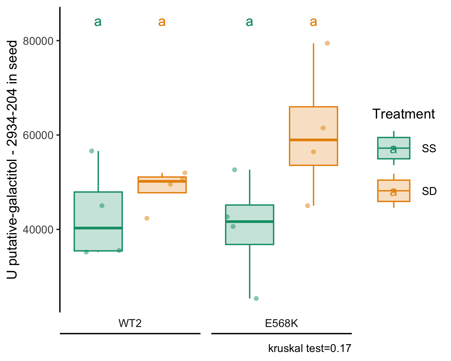
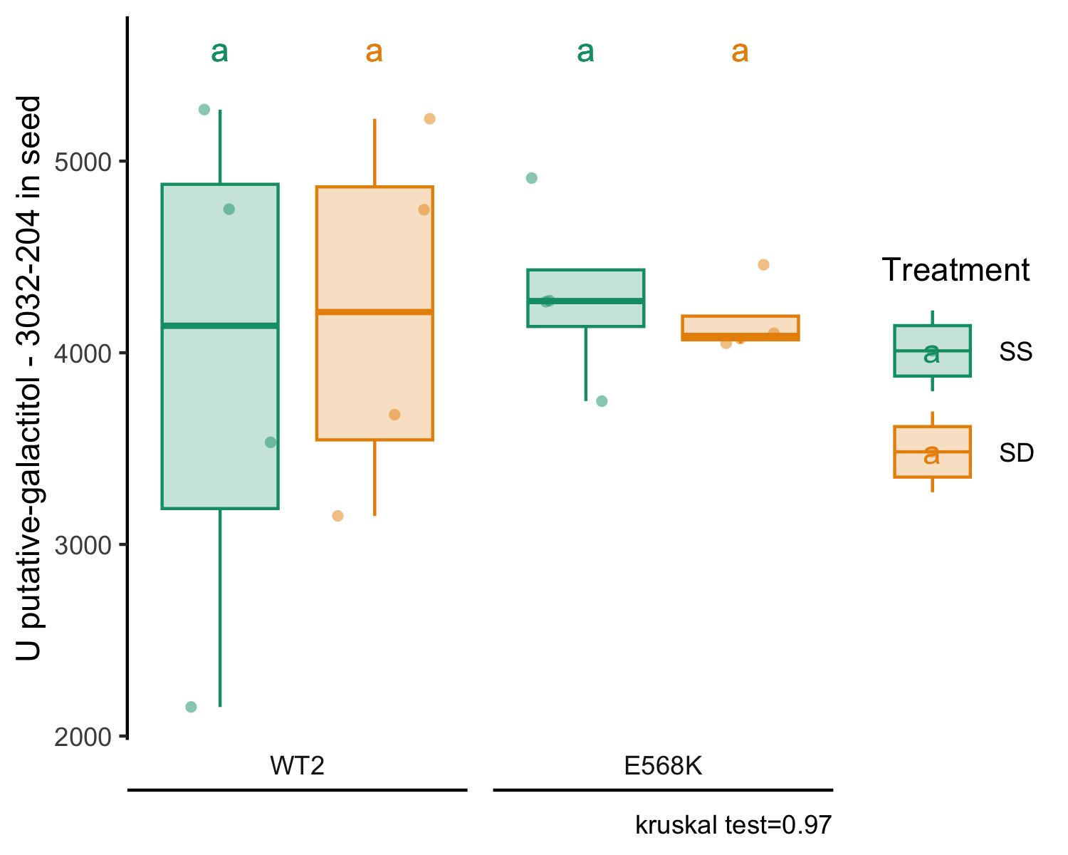
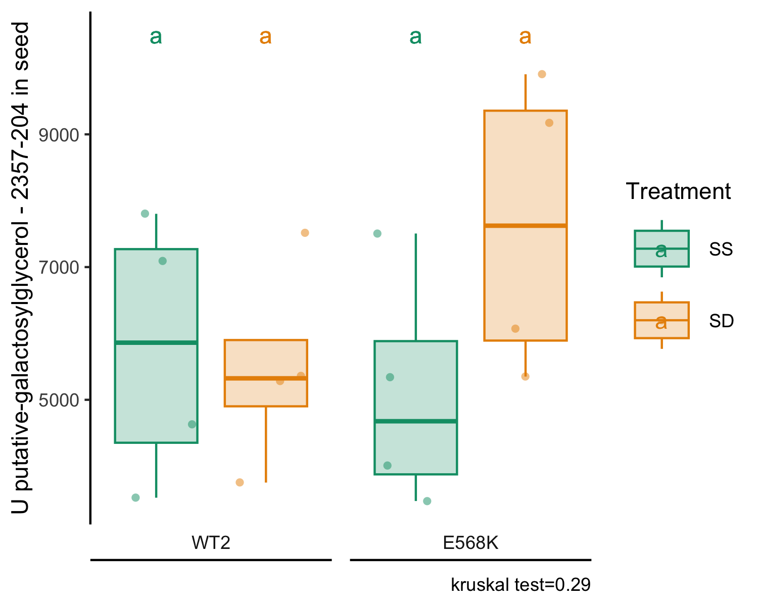
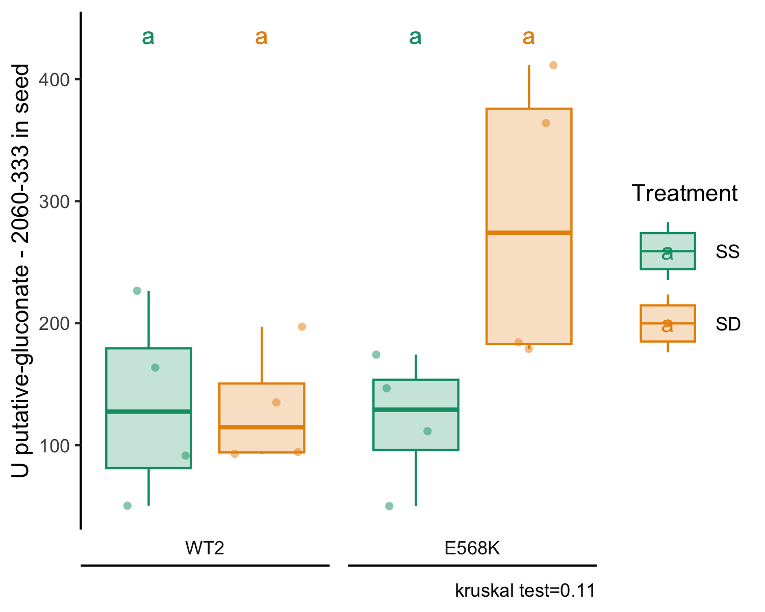
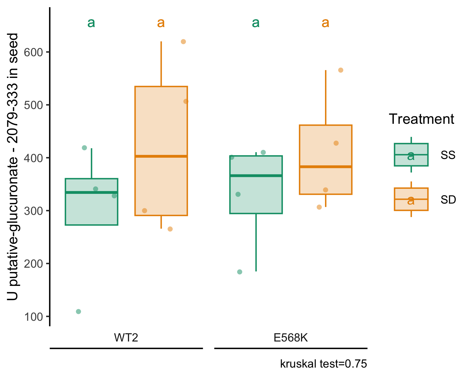
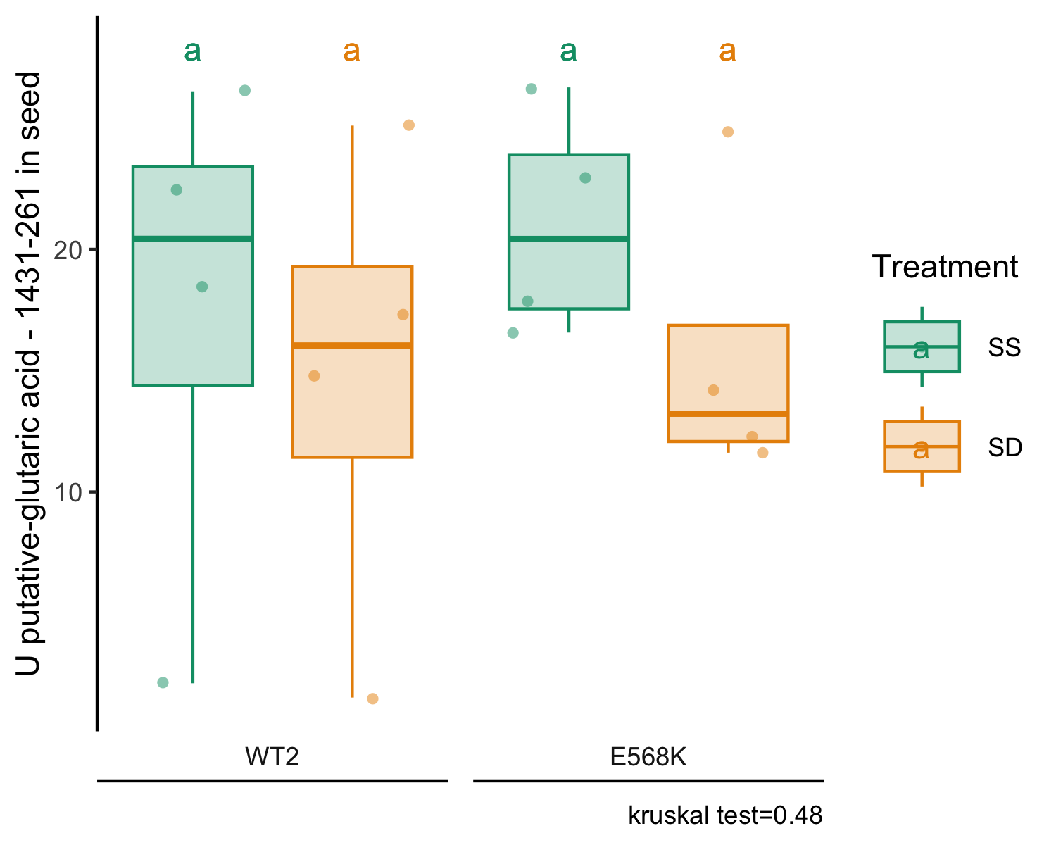
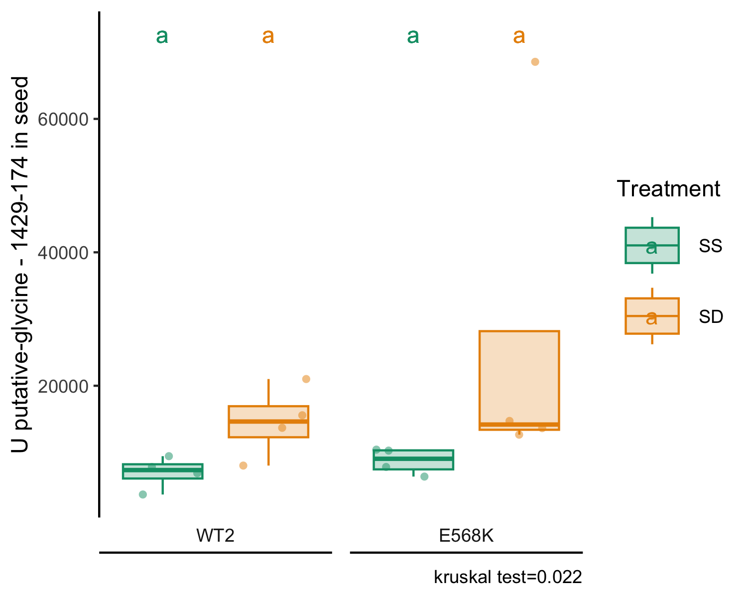
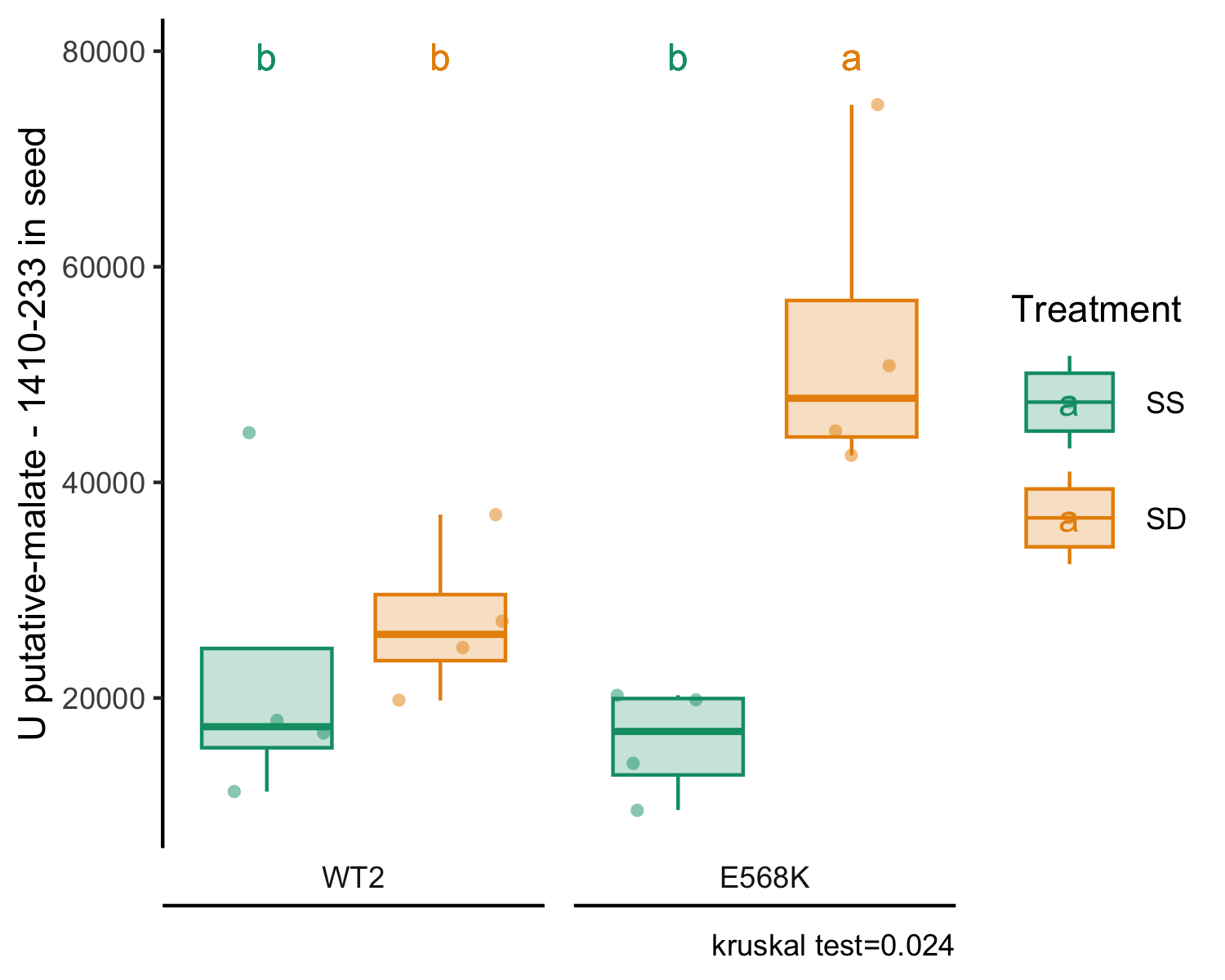
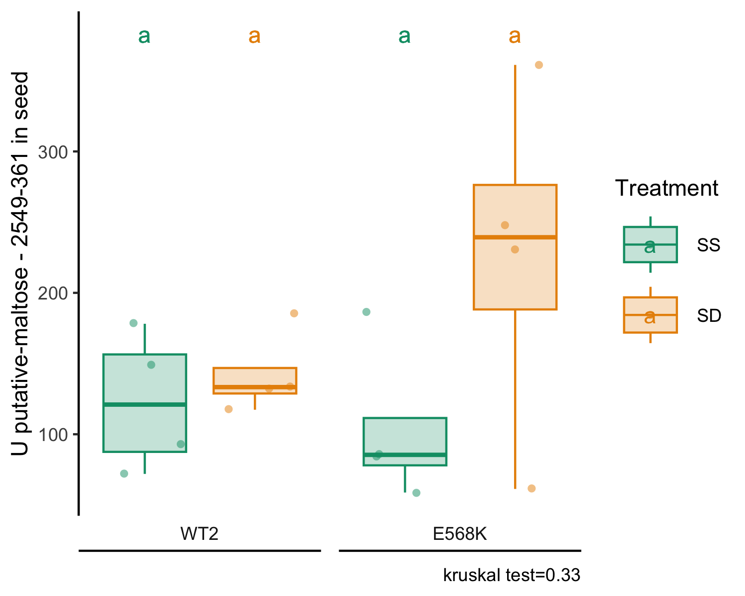
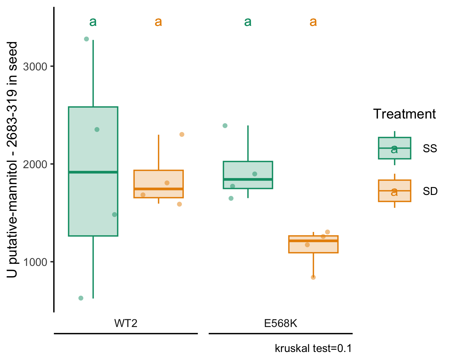
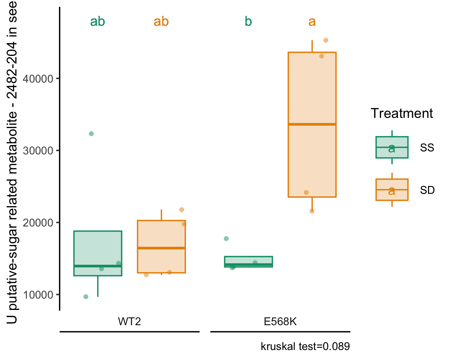
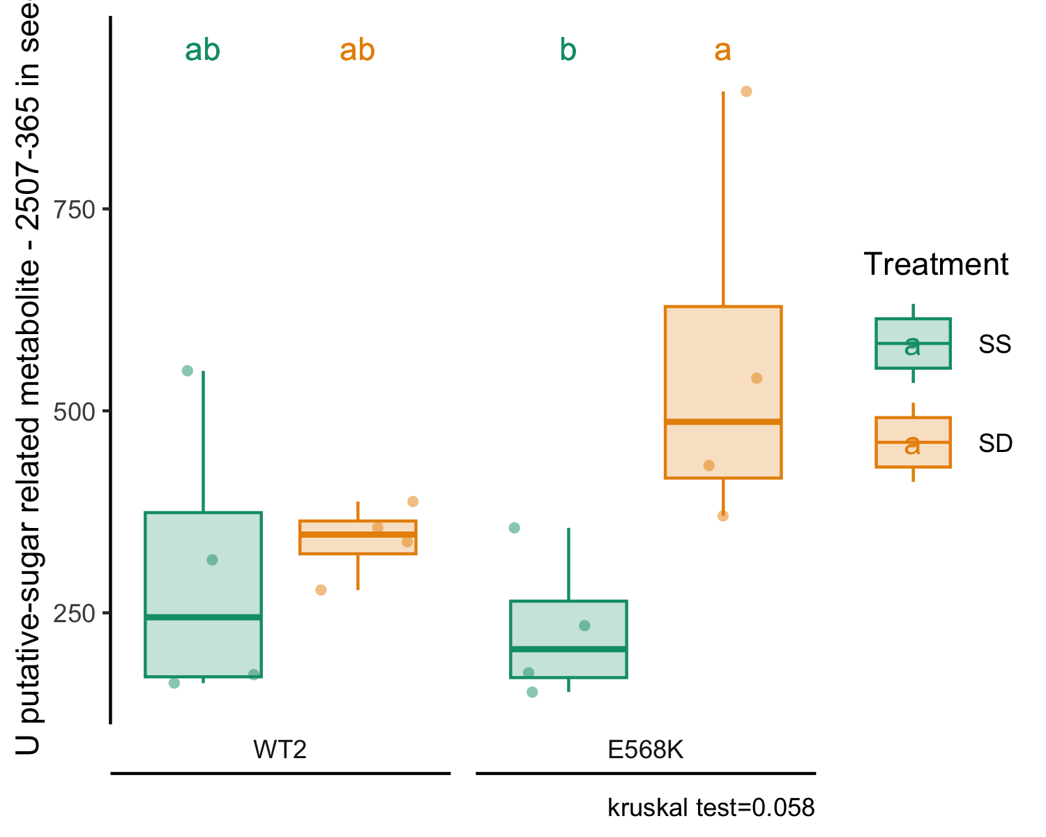
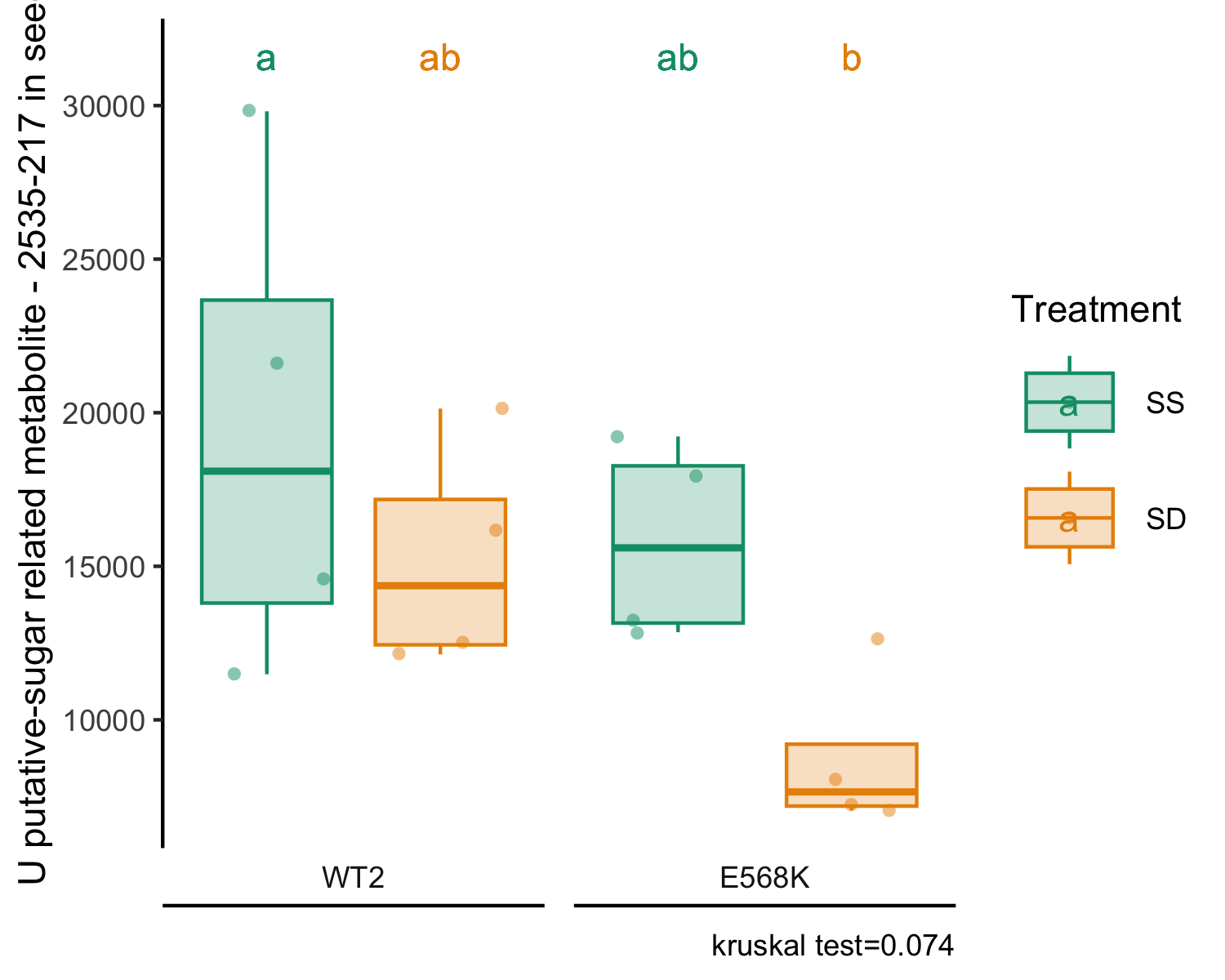
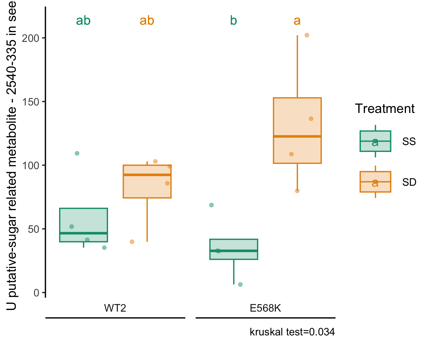
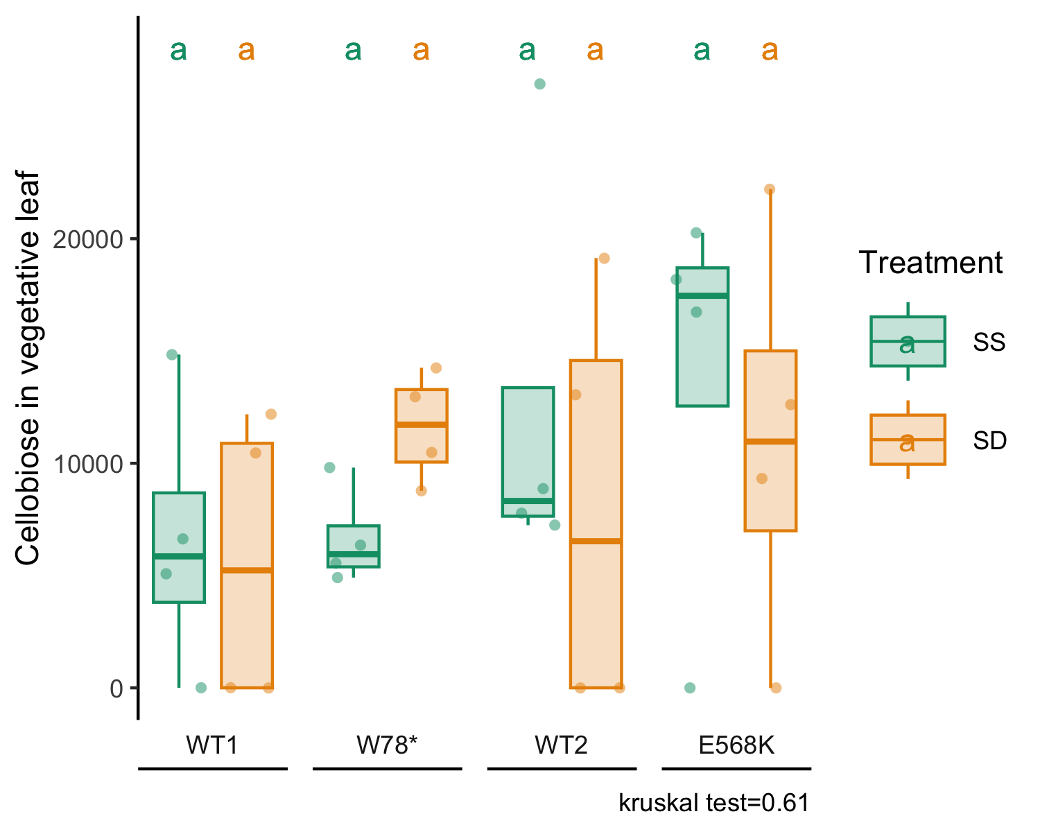
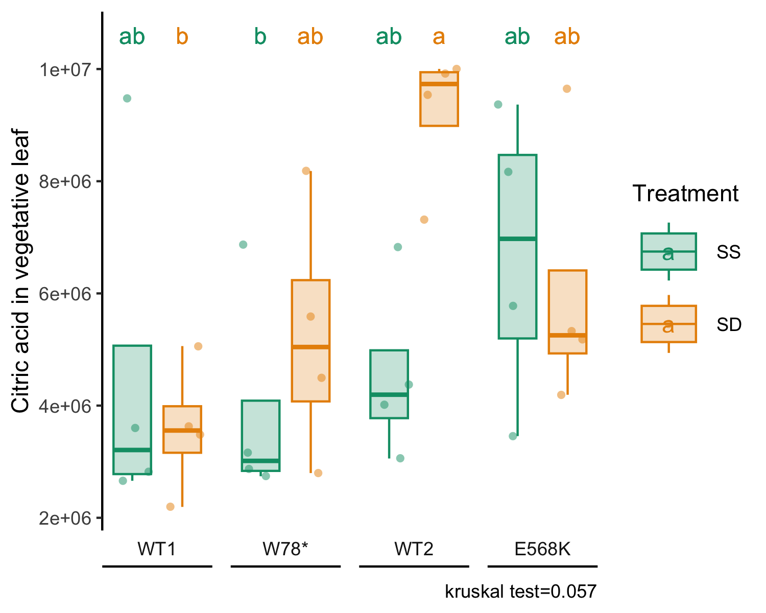
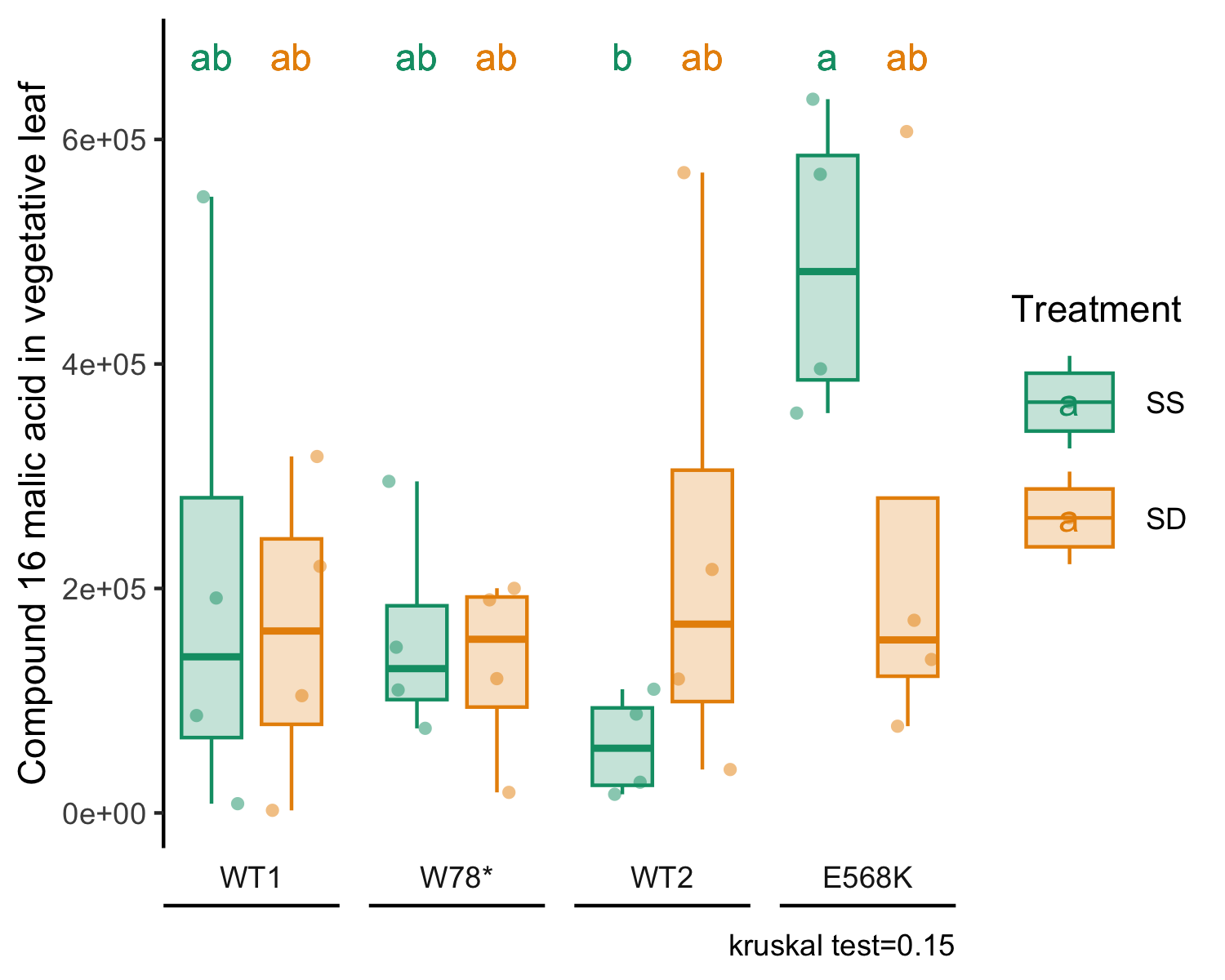
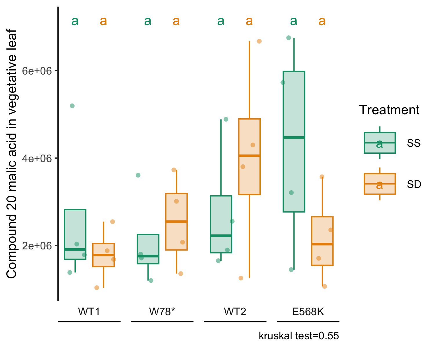
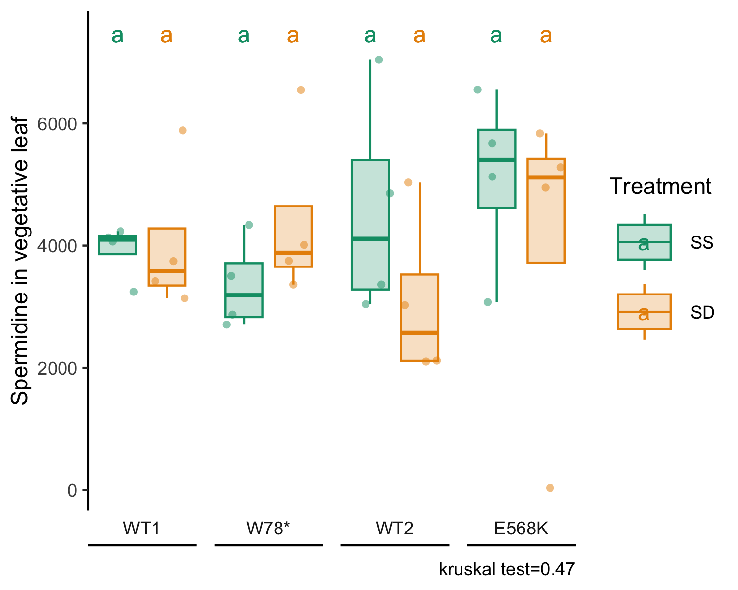
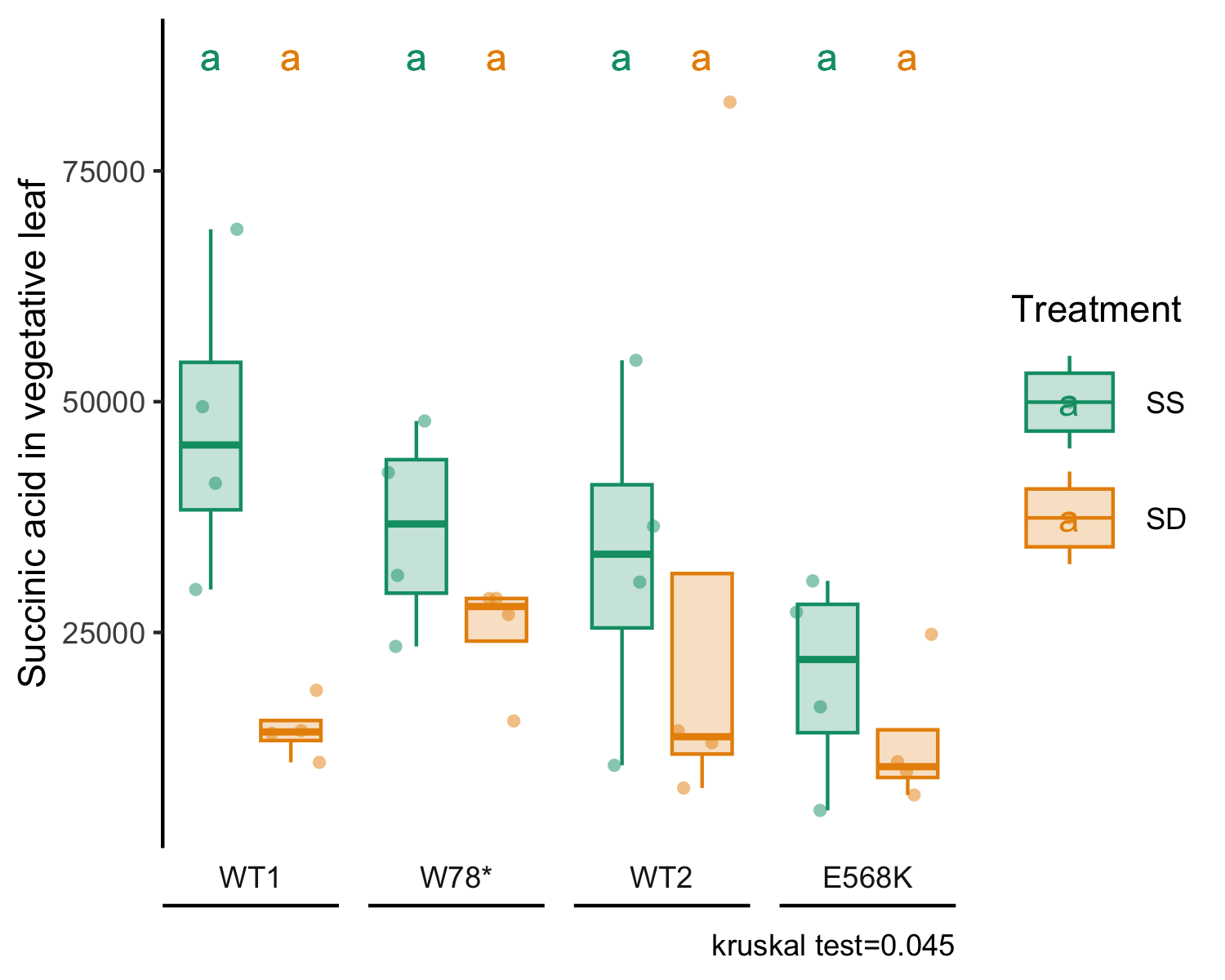
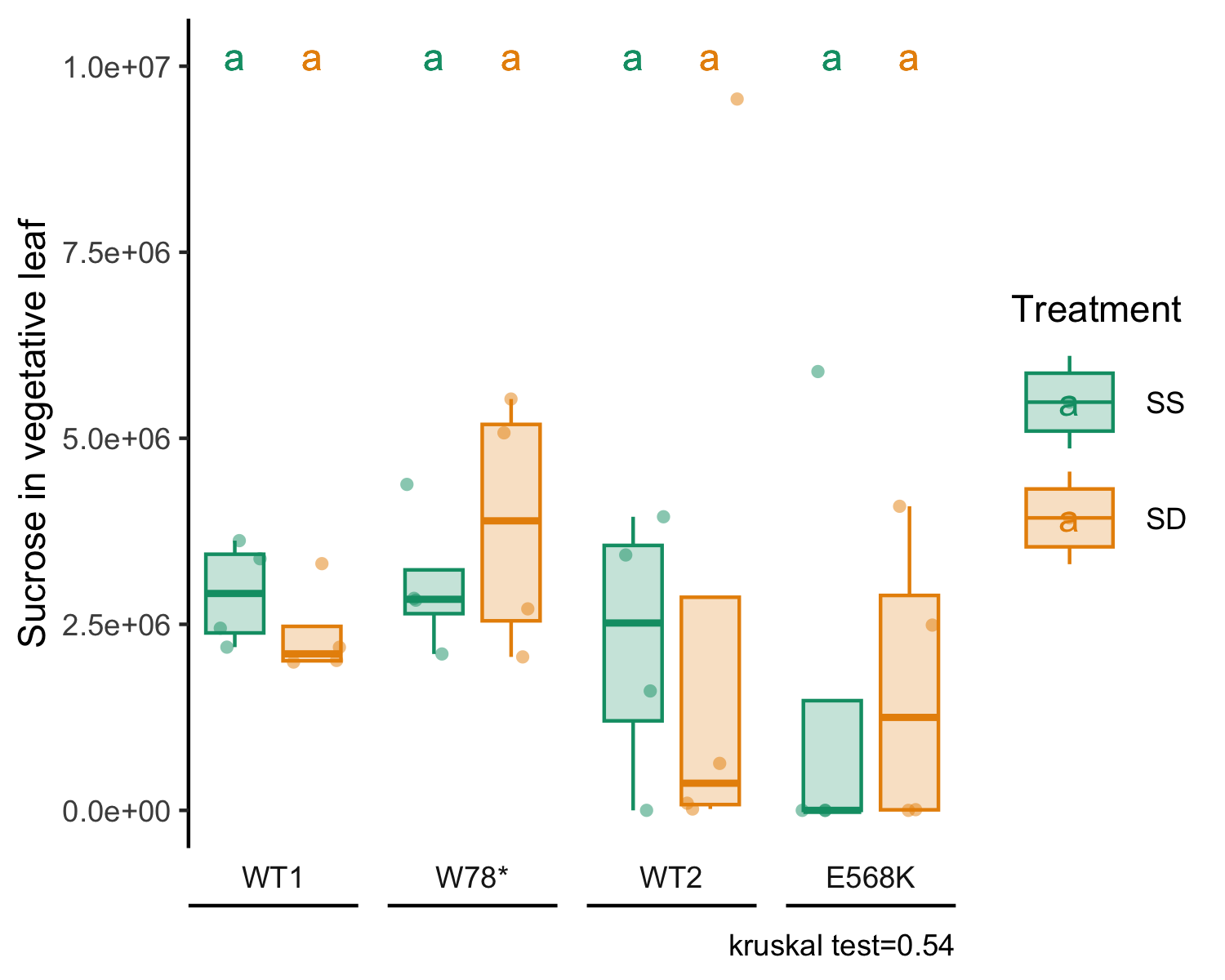
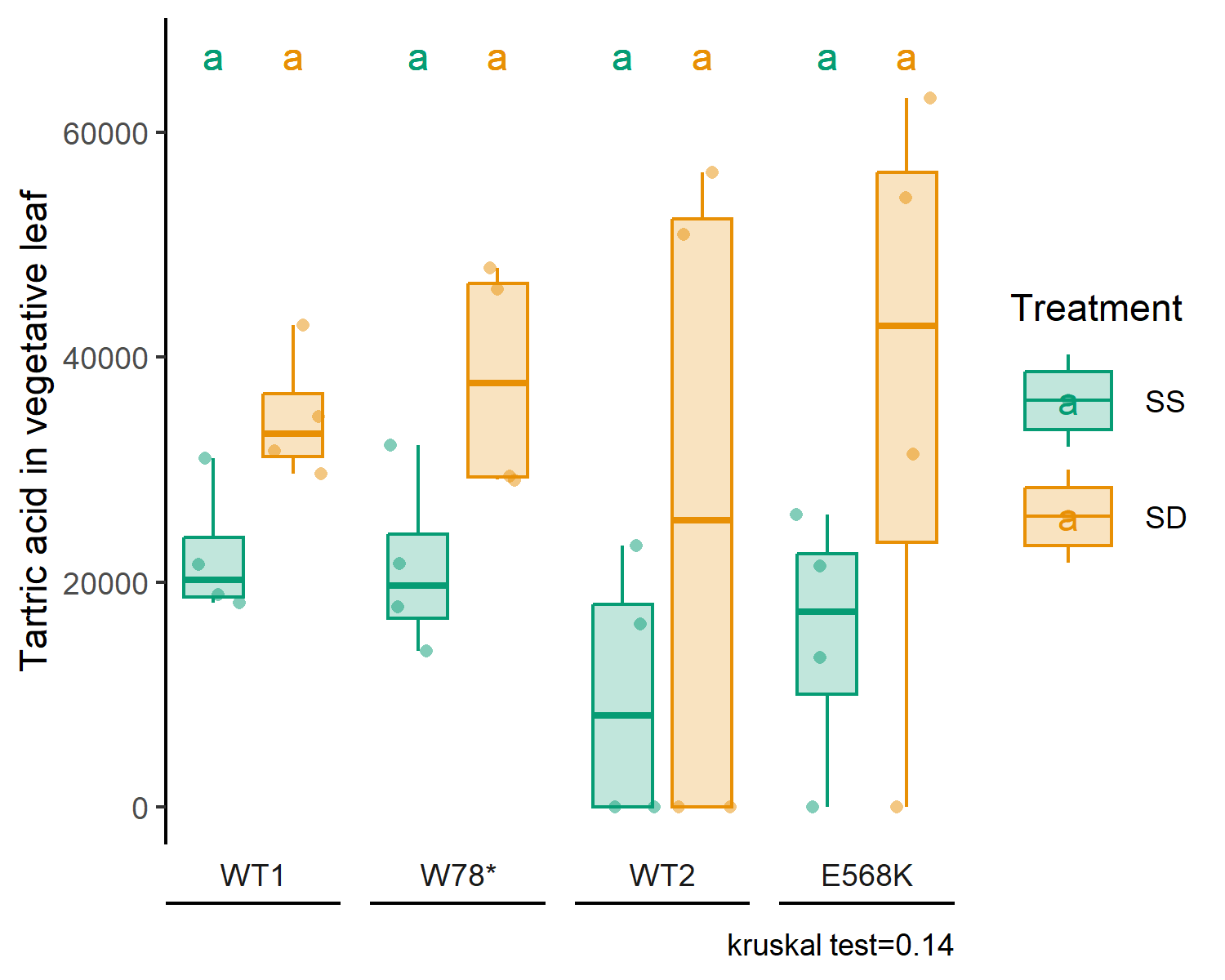
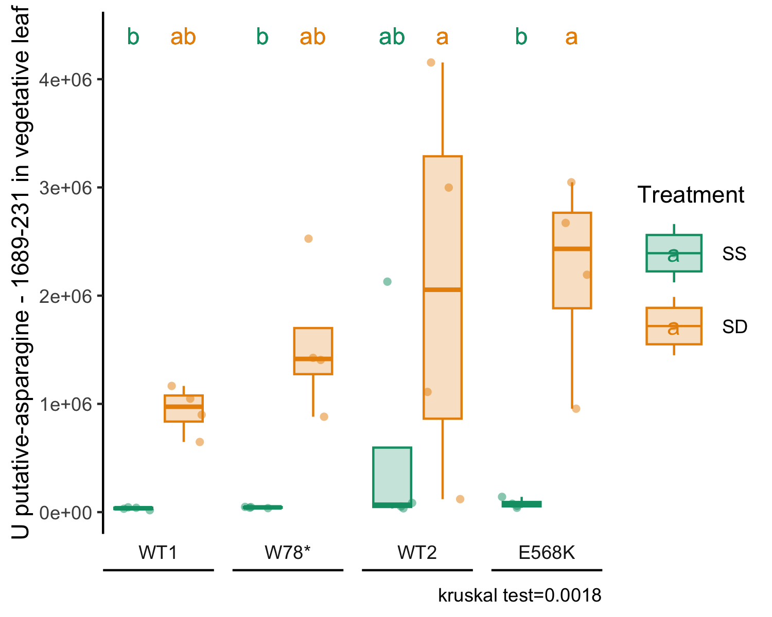
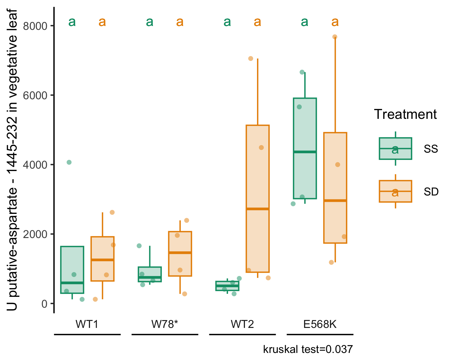
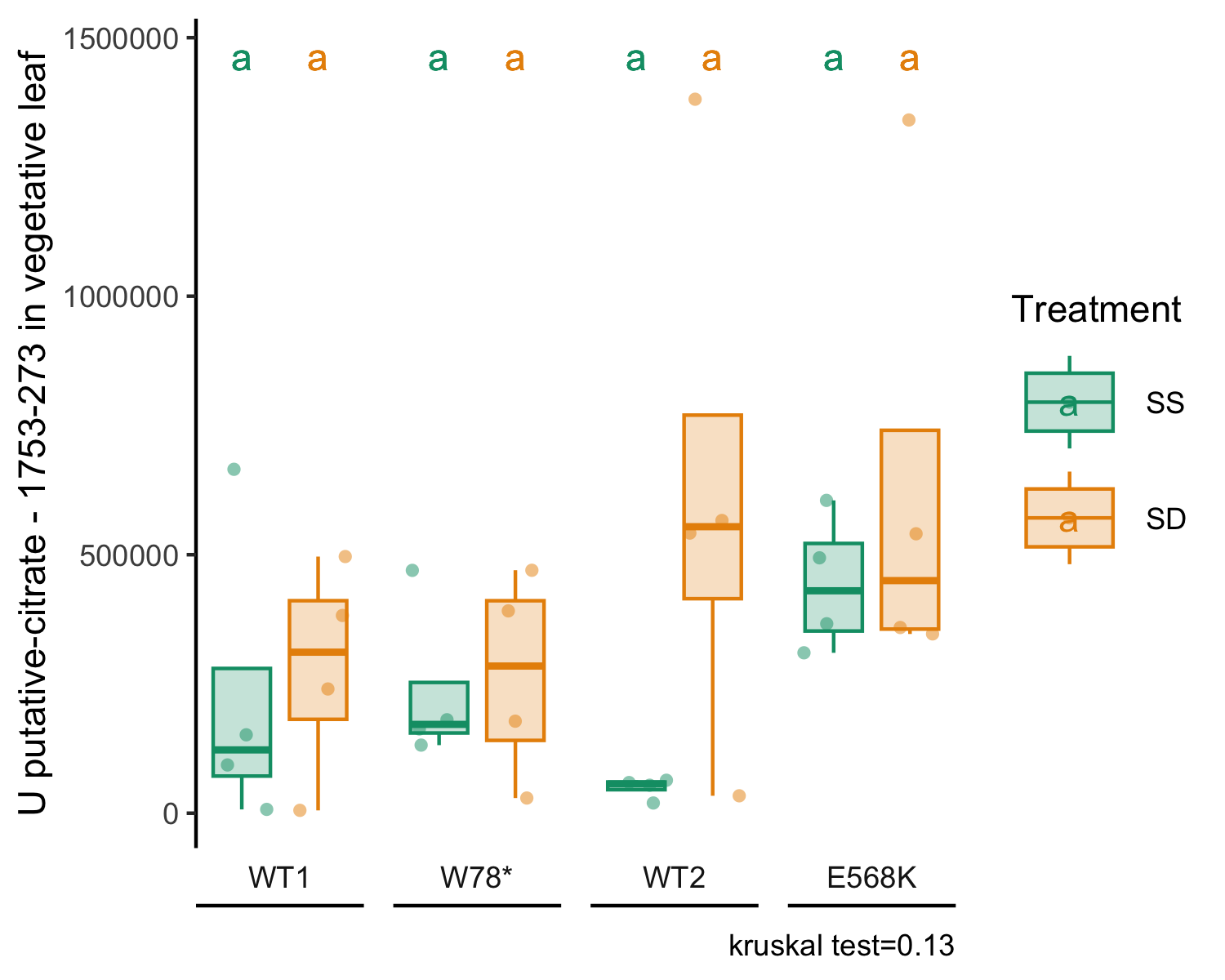
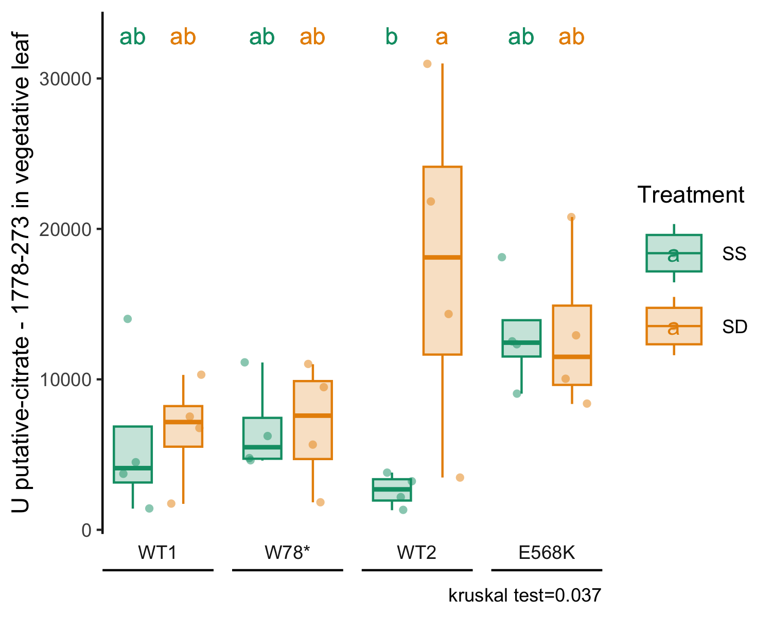
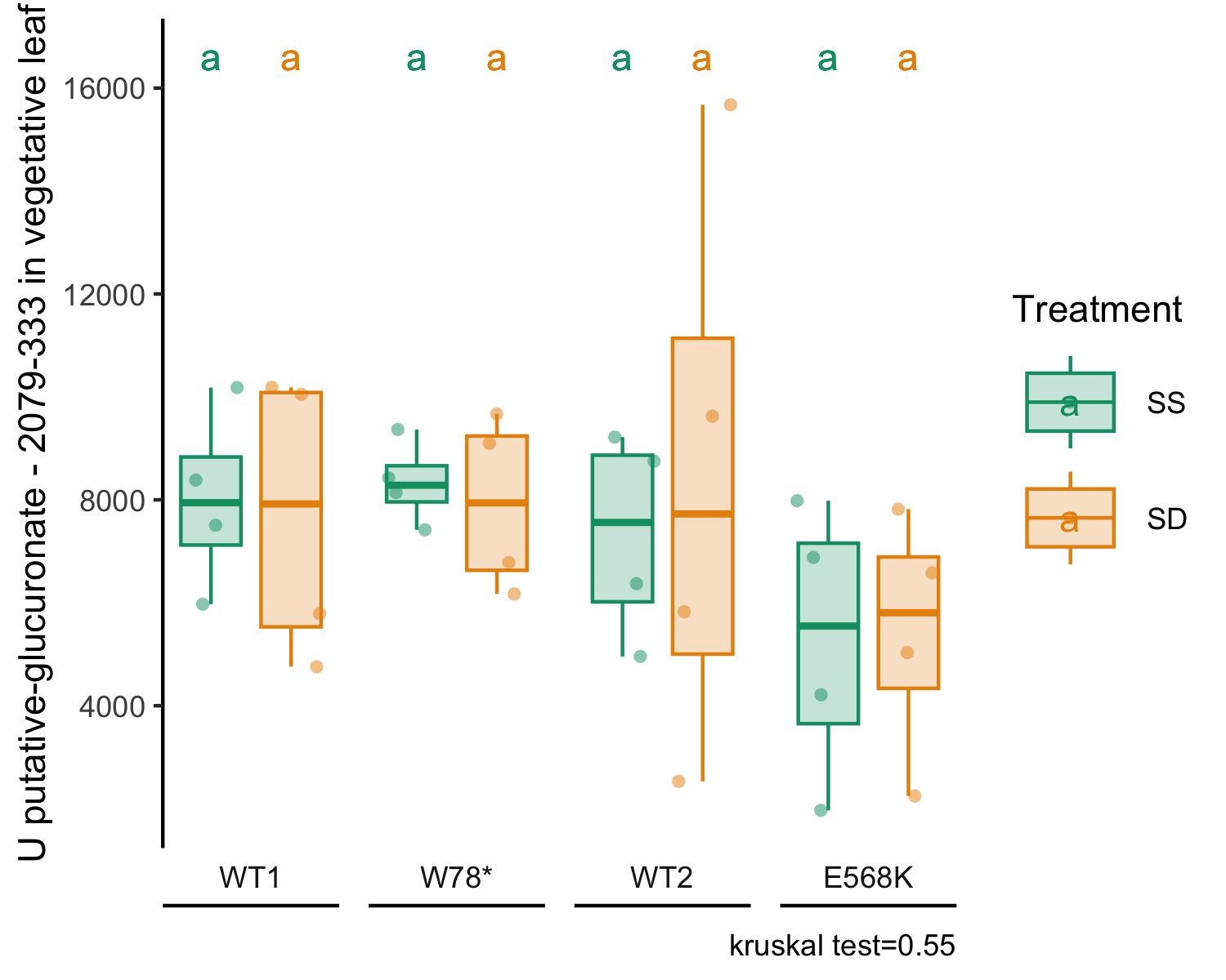
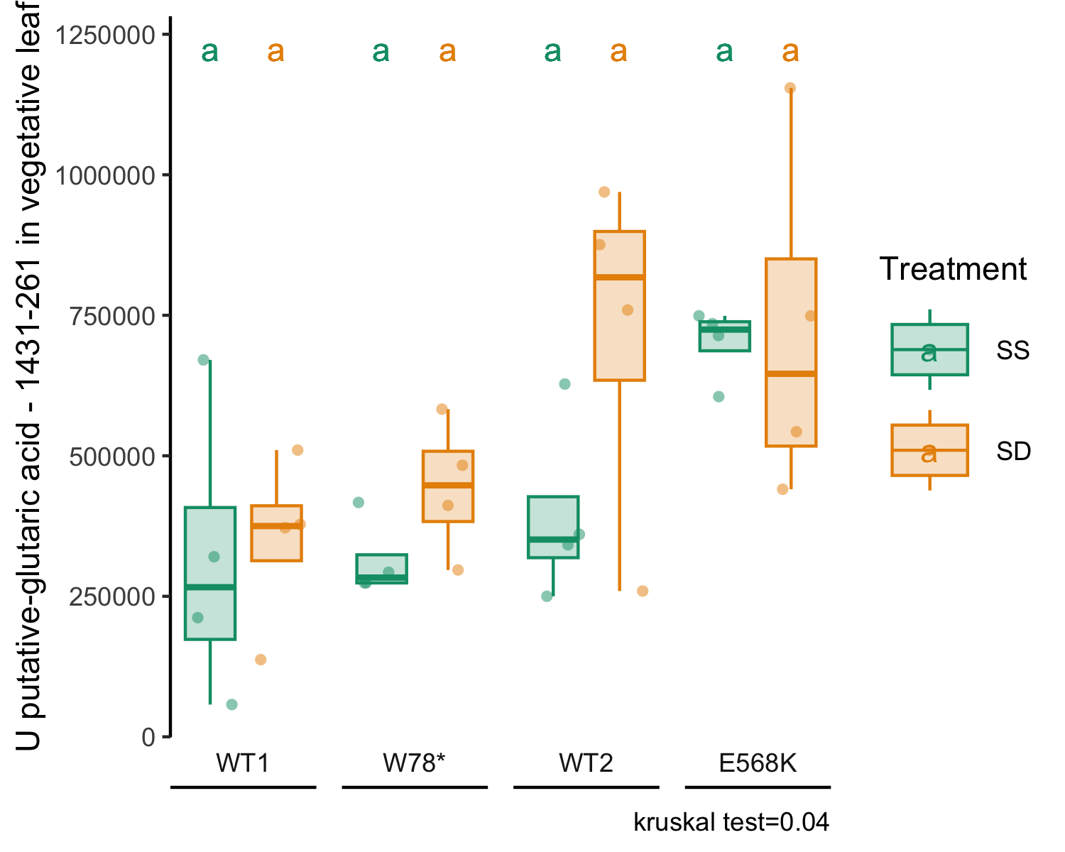
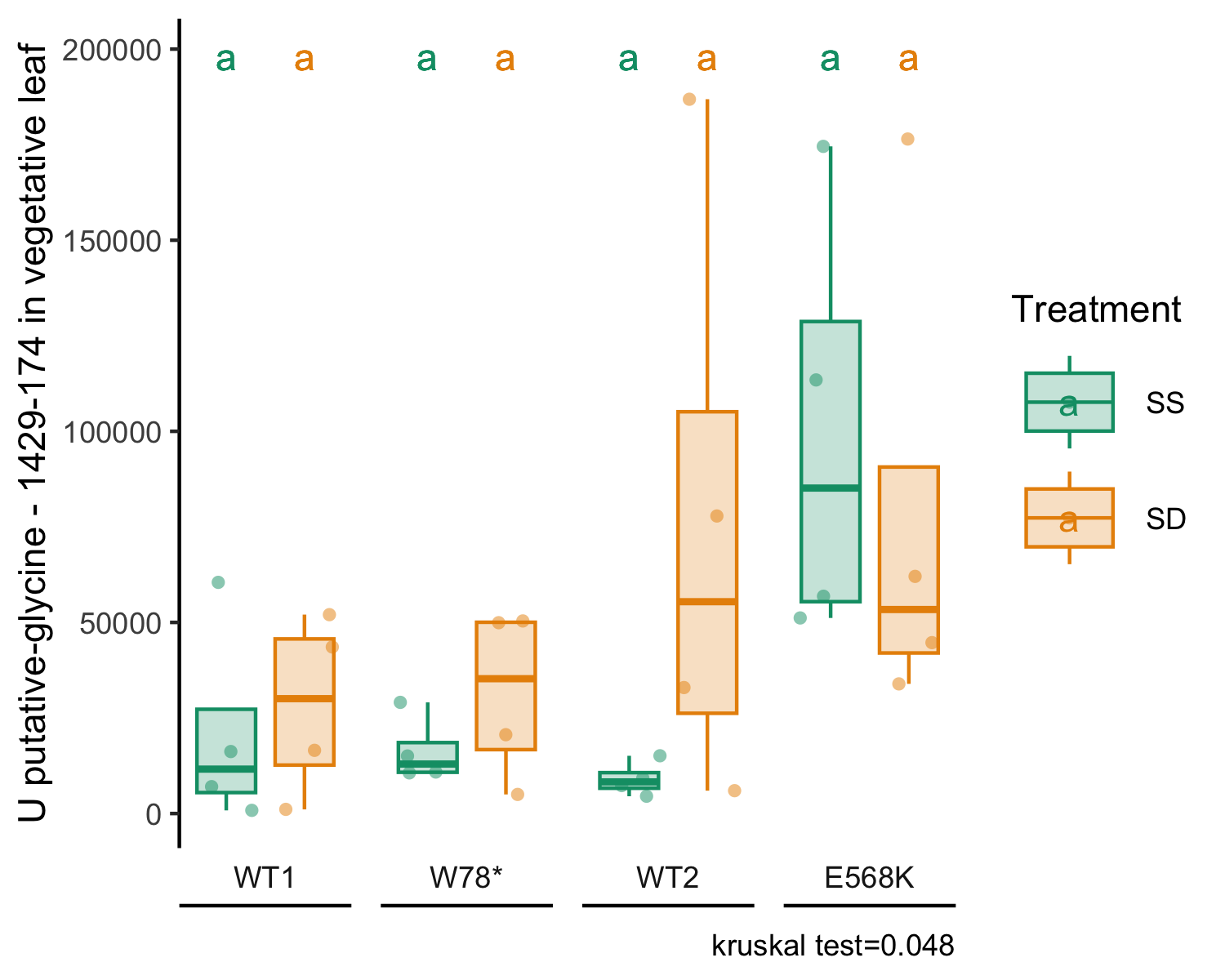
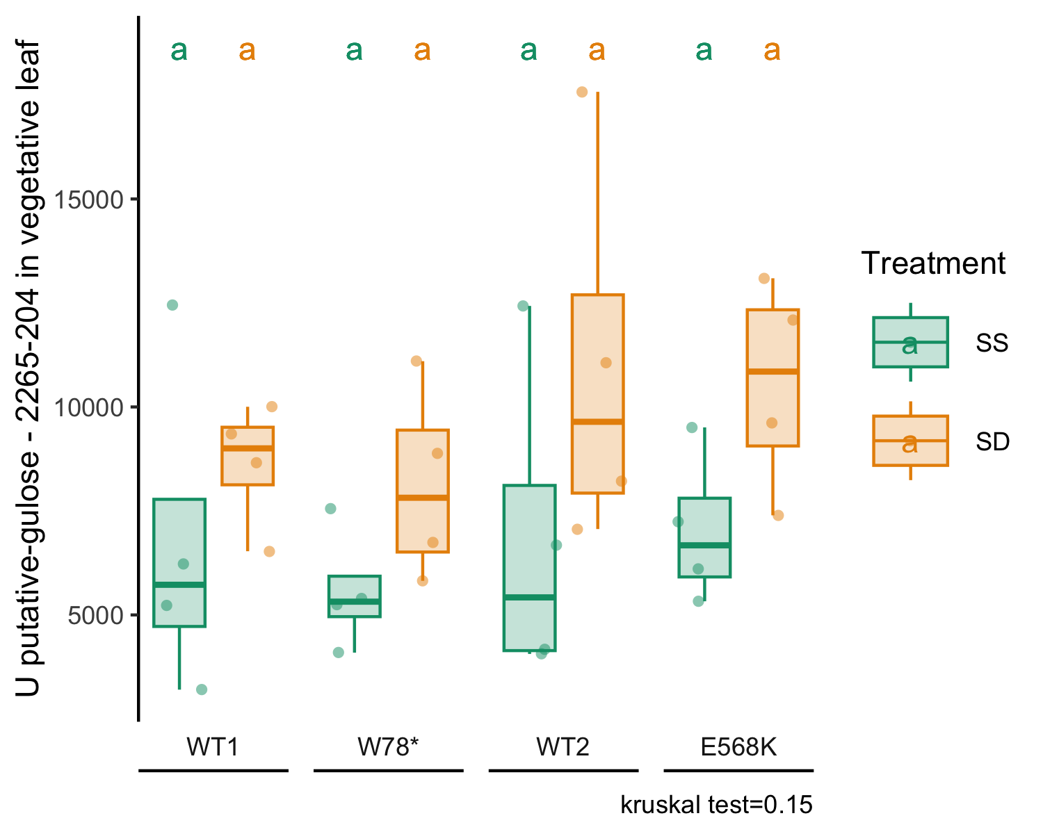
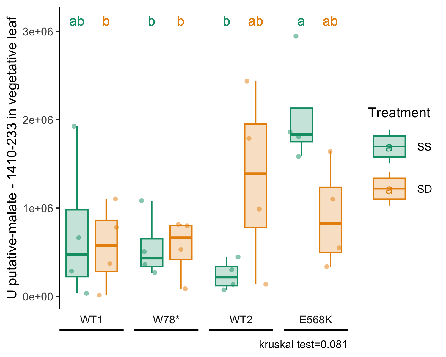
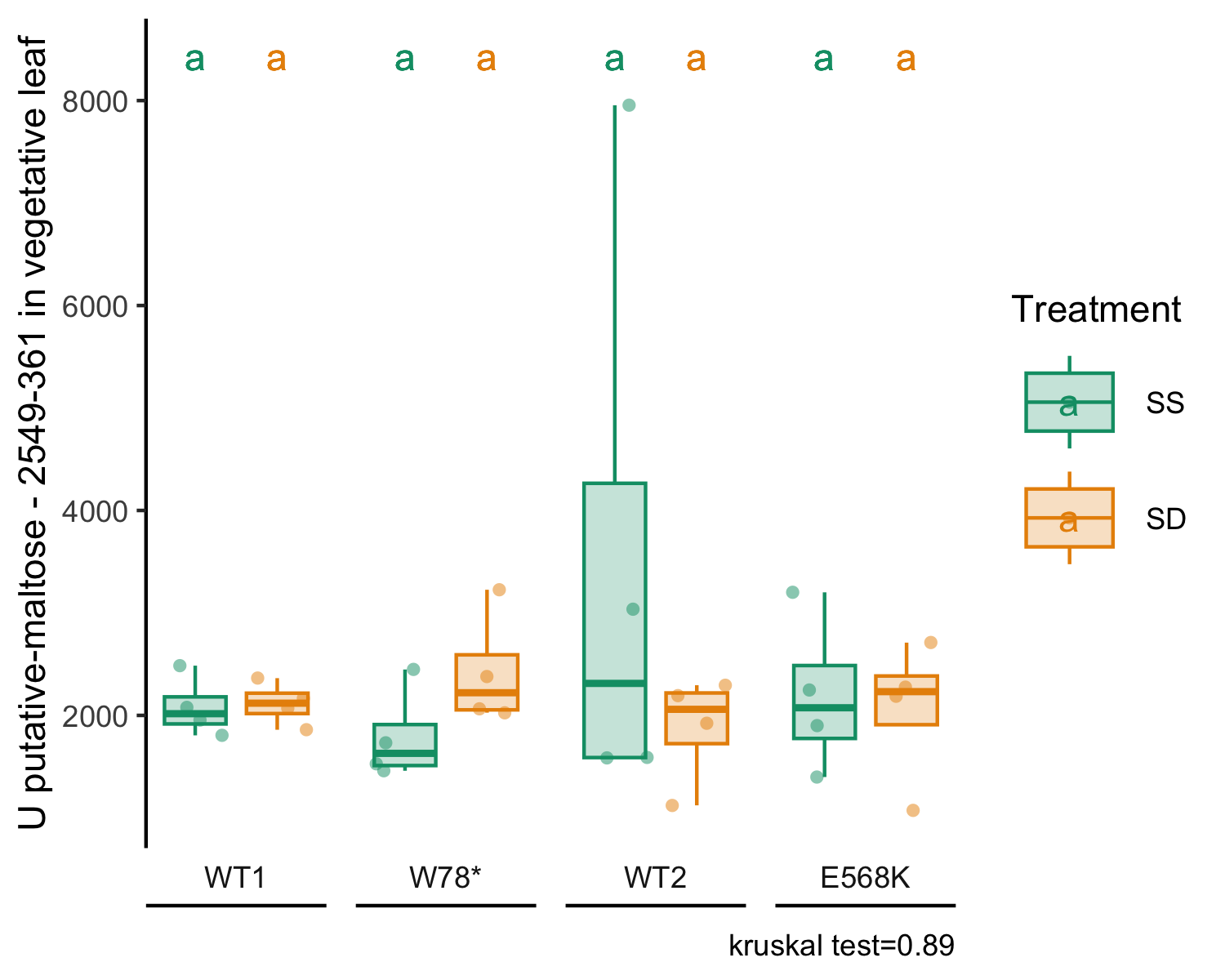
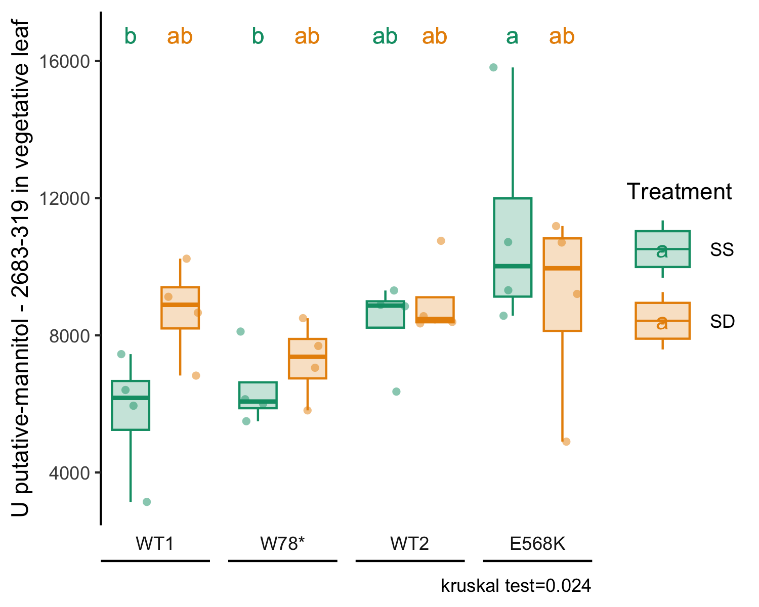
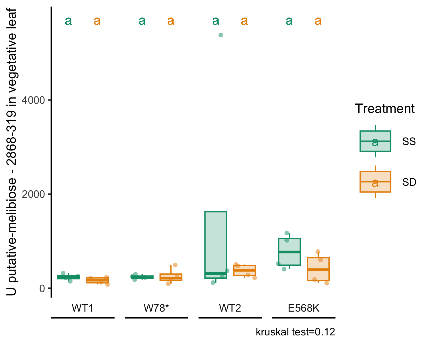
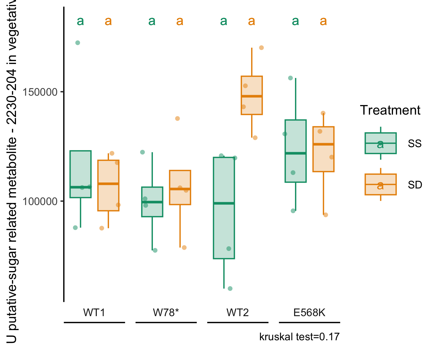
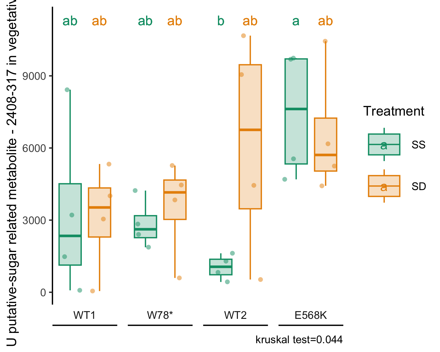
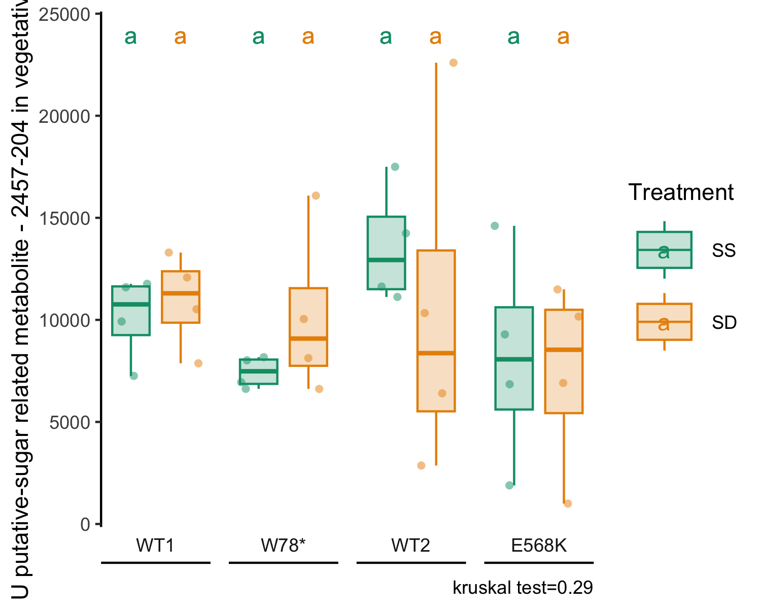
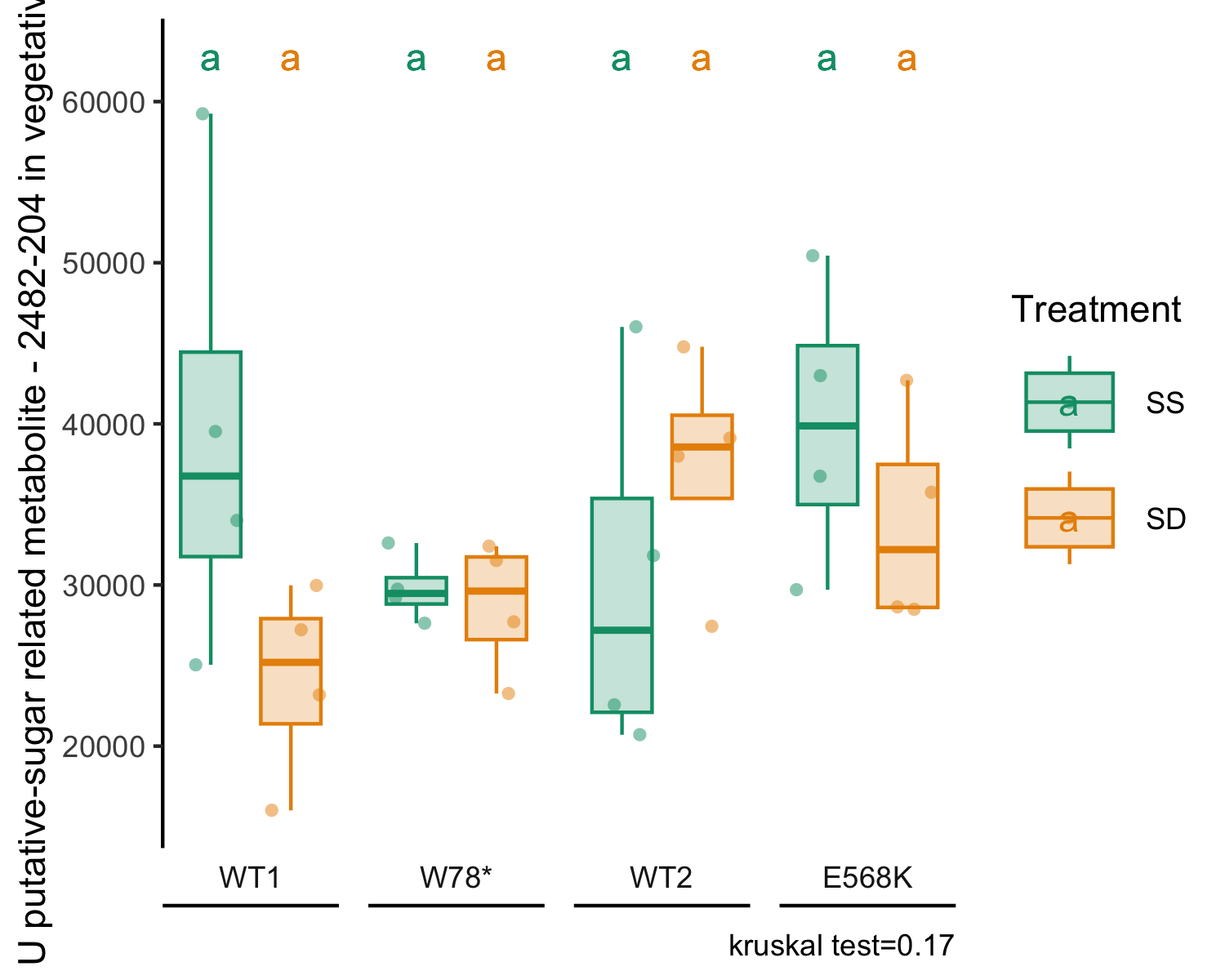
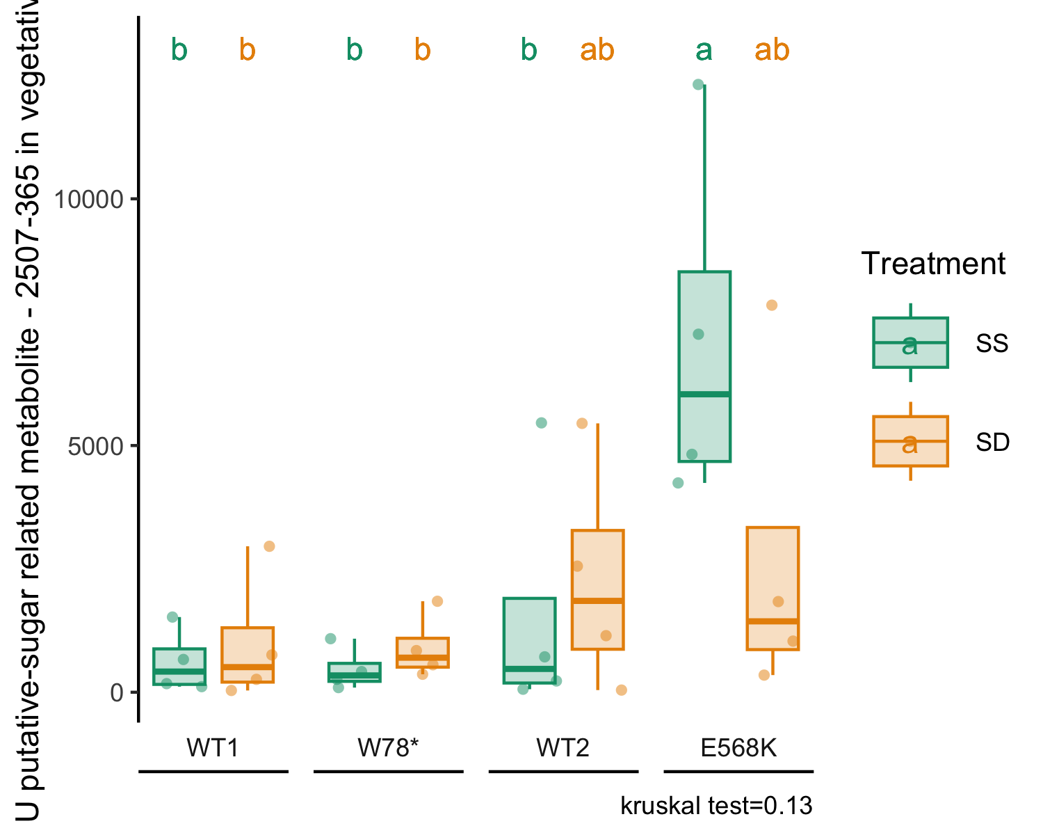
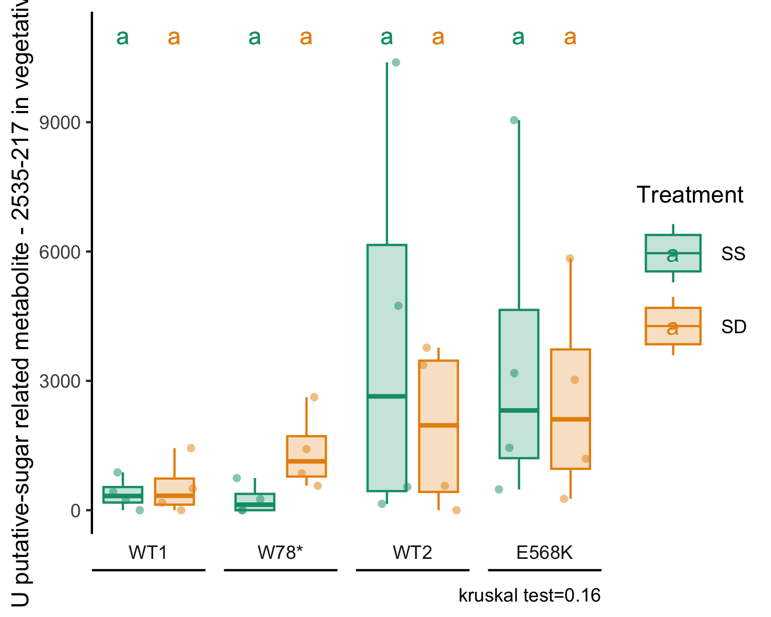
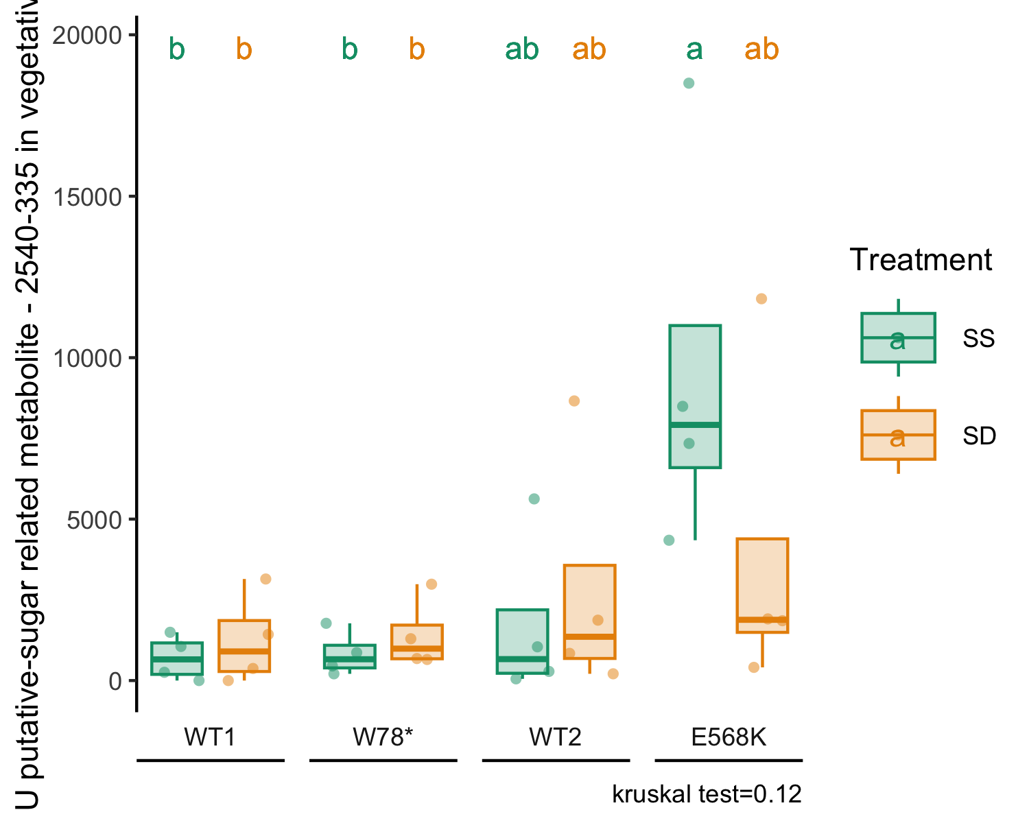
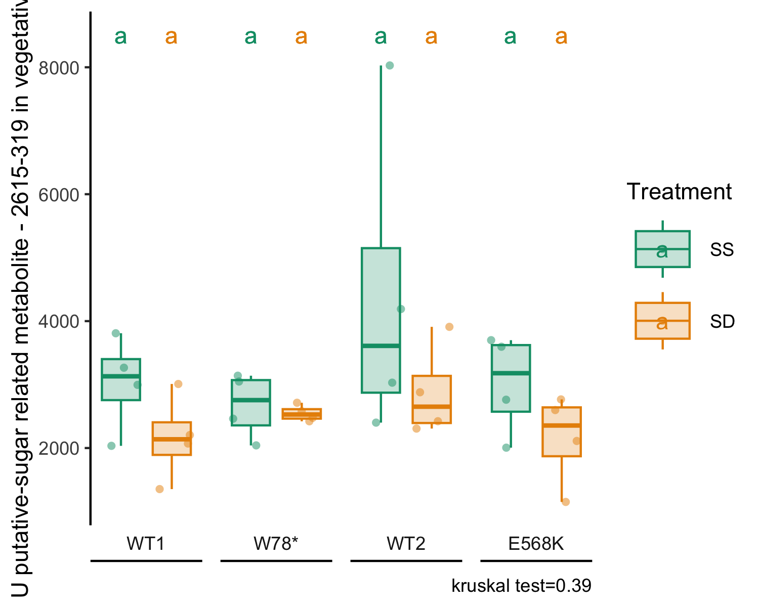
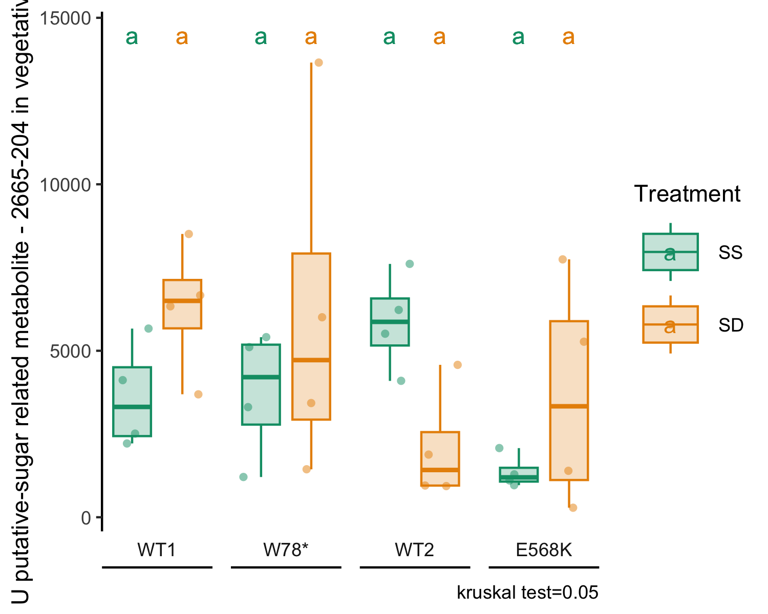
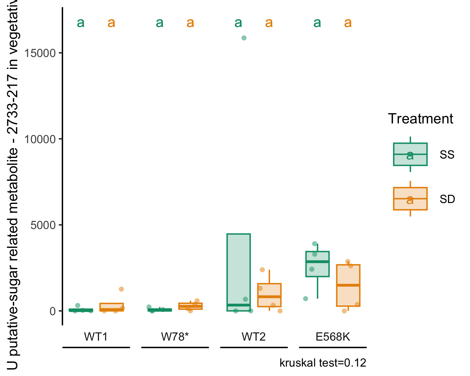
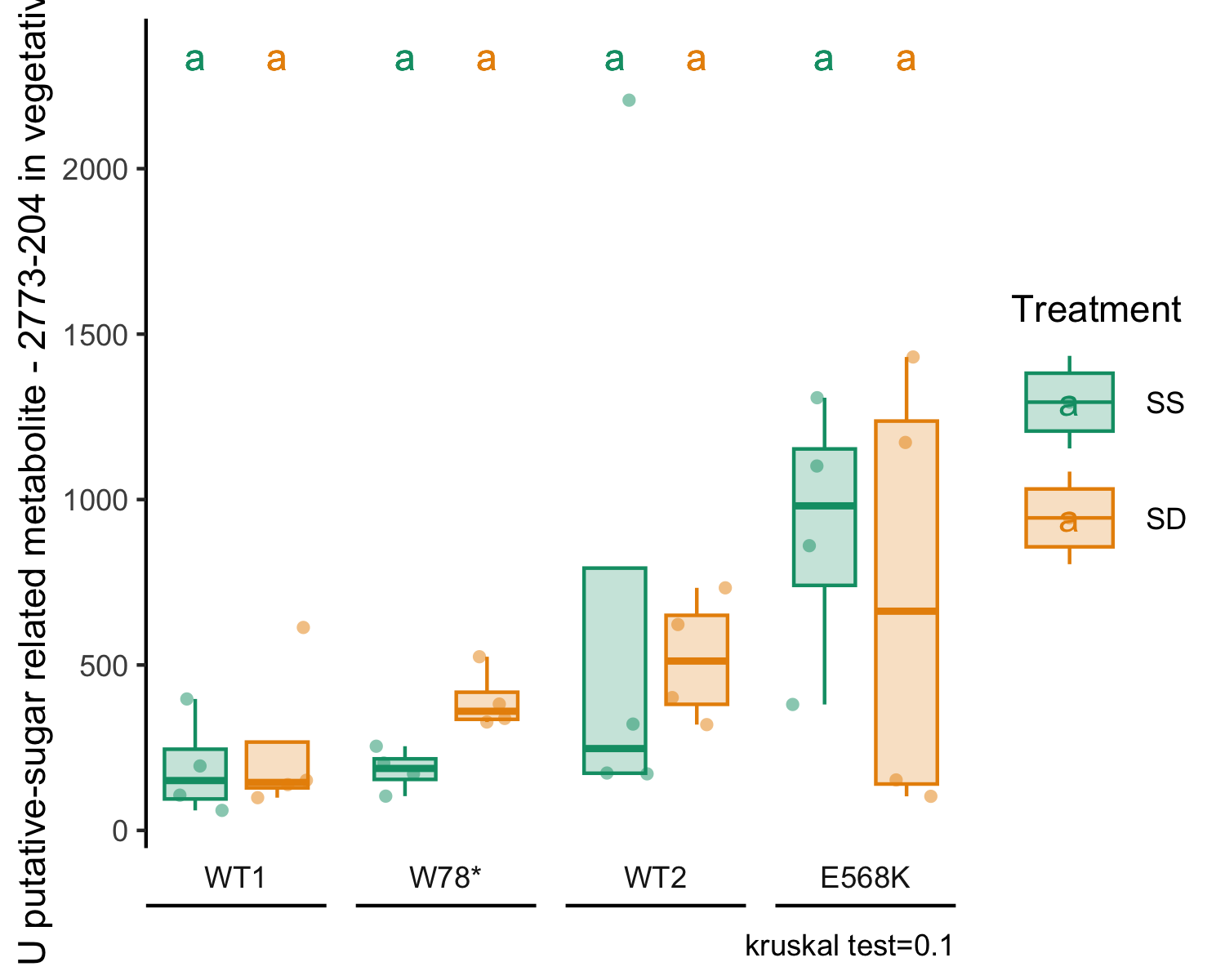
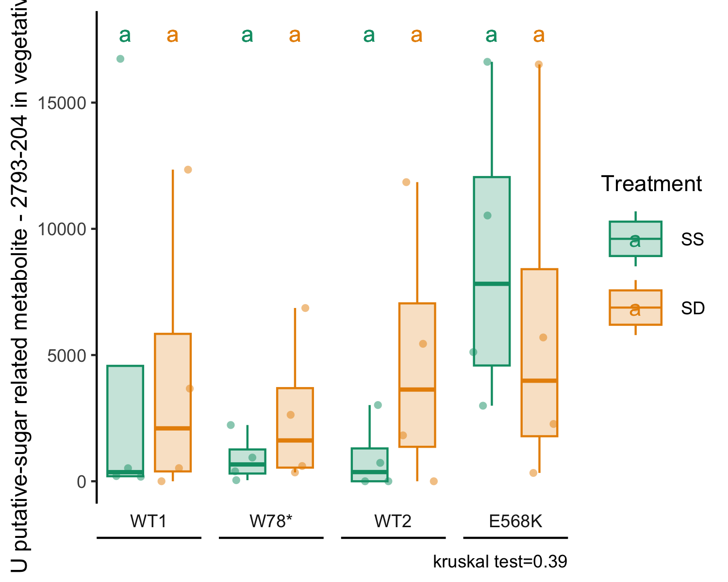
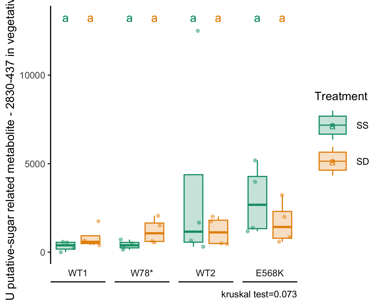
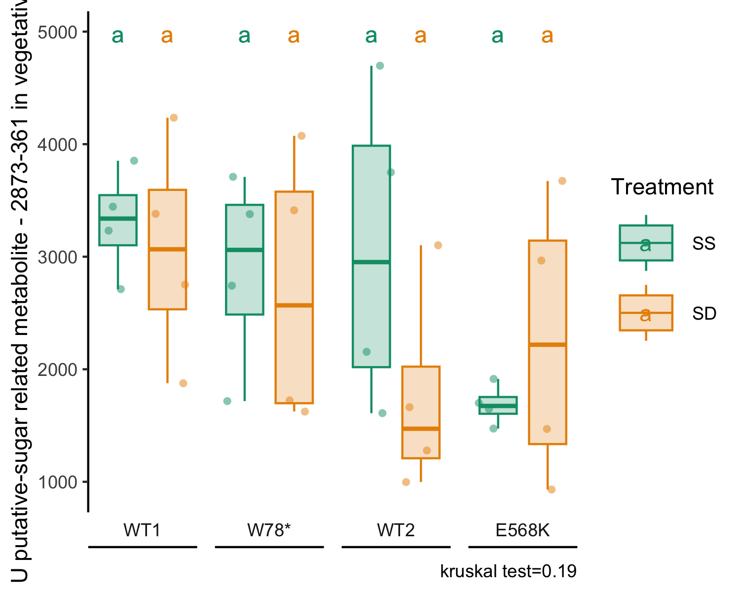
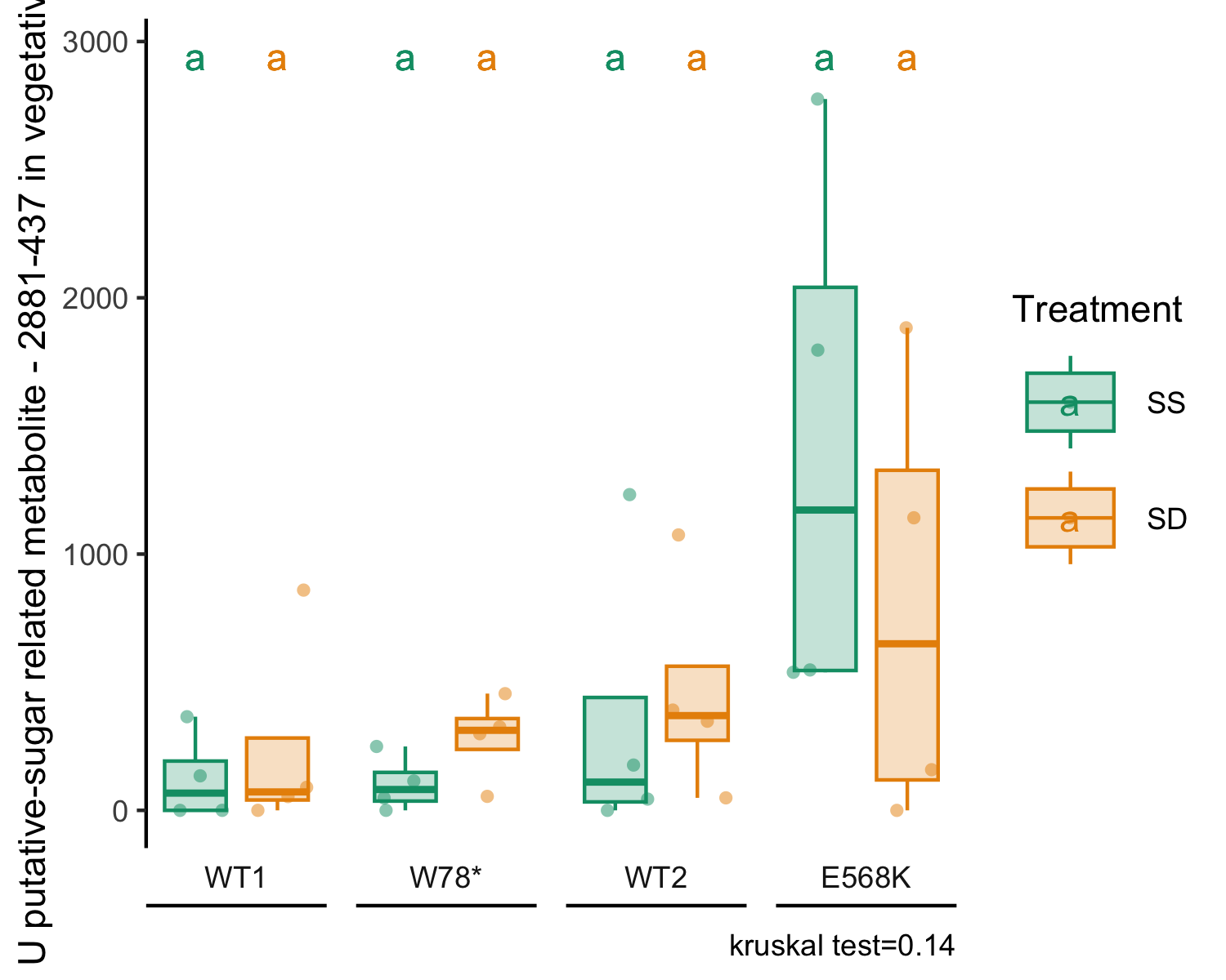
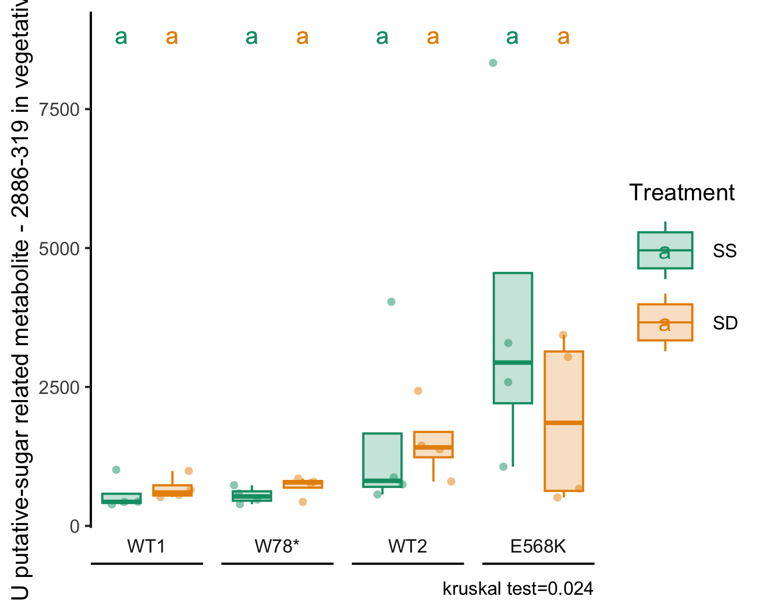
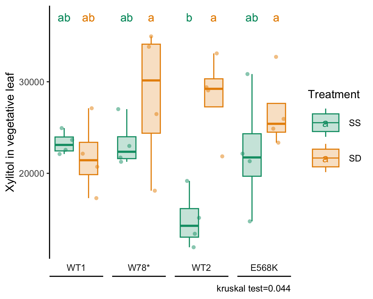
--- output: html_document editor_options: chunk_output_type: console --- ## Metabolomic from IBMP (2014) {#metabolomic} ```{r} #pkg library (mixOmics) # BiocManager::install("mixOmics") # plsda() library (readxl)library (tidyverse)library (ggnewscale) # to have two scale_fill library (ggh4x)library (kableExtra)library ("FactoMineR" )library ("factoextra" )library (patchwork)library (ggrepel) # nicer labels library (patchwork) # combine plots + shared legend library (glue) # tiny string helper library (pheatmap)# src source (here:: here ("src/function/stat_function/stat_analysis_main.R" )) # for make plot source (here:: here ("src/function/fig_export.R" )) # This function saves a given plot (plot_x) as both a PDF and a high-resolution PNG file at specified source (here:: here ("src/function/metabolomic/plot_plsda_compartment.R" )) # for make plot dimensions. # function <- function (string) {%>% str_replace_all ("_+" , " " ) %>% # replace one or more underscores by a space str_replace_all (":+" , " " ) %>% str_squish () %>% # remove any extra spaces str_to_sentence () # capitalize only the first letter # cosmetics = read_excel (here:: here ("data/color_palette.xlsm" )) %>% filter (set == "sulfure_condition" ) %>% :: select (color, treatment) %>% pull (color) %>% setNames (read_excel (here:: here ("data/color_palette.xlsm" )) %>% filter (set == "sulfure_condition" ) %>% pull (treatment)= read_excel (here:: here ("data/color_palette.xlsm" )) %>% filter (set == "mutant" ) %>% :: select (color, treatment) %>% pull (color) %>% setNames (read_excel (here:: here ("data/color_palette.xlsm" )) %>% filter (set == "mutant" ) %>% pull (treatment)``` ## Data importation ## The sample from vegetative leaves from plant 60 was removed due to the high PLSDA. ```{r, eval = F} df_info_seed <- read_excel(here::here("data/plant_info_XP2013.xlsx")) %>% dplyr::select(!c("comment", "tablar position", "row", "line", "tablar", "greenhouse")) df_metabo_seed = read_excel(here::here("data/metabolomic/raw_IBMP_201409_untargeted.xlsx")) %>% dplyr::select(!c("Internal standard","ID_2","ID_3","ID_4","Sample")) %>% dplyr::rename(compartment = "ID_1", number_XP = ID_5) %>% filter(compartment == "graine") %>% mutate(compartment = "seed") %>% full_join(., df_info_seed, by = "number_XP") %>% dplyr::select(-matches("Compound"), matches("Compound")) df_metabo_leaf = read_excel(here::here("data/metabolomic/raw_IBMP_201409_untargeted.xlsx")) %>% dplyr::select(!c("Internal standard", "ID_2","ID_3","ID_4","Sample")) %>% dplyr::rename(compartment = "ID_1", number_XP = ID_5) %>% filter(compartment != "graine") %>% mutate(compartment = fct_recode(compartment, "reproductive leaf" = "feuille reproductrice", "vegetative leaf" = "feuille végétative")) # for repro df_info_leaf_repro <- read_excel(here::here("data/plant_info_XP2014.xlsx")) %>% dplyr::select(-c(number_XP, code_metabo_leaf_vege, code_run_transcripto, code_transcripto, "tablar position", "comment", "line", "row", "plant_spad", "osmometer", "greenhouse", "tablar")) %>% drop_na(code_metabo_leaf_repro) %>% dplyr::rename(number_XP = code_metabo_leaf_repro) df_metabo_leaf_repro <- df_metabo_leaf %>% filter(compartment == "reproductive leaf") %>% full_join(., df_info_leaf_repro, by = "number_XP") %>% dplyr::select(-matches("Compound"), matches("Compound")) # for vege df_info_leaf_vege <- read_excel(here::here("data/plant_info_XP2014.xlsx")) %>% dplyr::select(-c(number_XP, code_metabo_leaf_repro, code_run_transcripto, code_transcripto, "tablar position", "comment", "line", "row", "plant_spad", "osmometer", "greenhouse", "tablar")) %>% drop_na(code_metabo_leaf_vege) %>% dplyr::rename(number_XP = code_metabo_leaf_vege) df_metabo_leaf_vege <- df_metabo_leaf %>% filter(compartment == "vegetative leaf") %>% full_join(., df_info_leaf_vege, by = "number_XP") %>% dplyr::select(-matches("Compound"), matches("Compound")) %>% filter(plant_num != 60) df_metabolite_global <- bind_rows(df_metabo_leaf_repro, df_metabo_leaf_vege, df_metabo_seed) %>% mutate( type_genotype = ifelse(genotype %in% c("WT1", "WT2"), "WT", "Mut") ) %>% pivot_longer( cols = starts_with("Compound"), names_to = "variable_originale", values_to = "value" ) # 2. Tu crées une version "propre" des noms en enlevant "Compound XX:" df_metabolite_global <- df_metabolite_global %>% mutate(variable_propre = str_remove(variable_originale, "^Compound \\d+:\\s*")) # 3. Tu regardes où il y a des doublons dans les noms "propres" variables_avec_doublon <- df_metabolite_global %>% distinct(variable_originale, variable_propre) %>% dplyr::count(variable_propre) %>% filter(n > 1) %>% pull(variable_propre) # 4. Si la version propre est un doublon, tu gardes le nom original df_metabolite_global <- df_metabolite_global %>% mutate( variable = if_else(variable_propre %in% variables_avec_doublon, variable_originale, variable_propre) ) # 5. Tu continues ton traitement normal df_metabolite_global <- df_metabolite_global %>% mutate( sulfur_condition = fct_relevel(sulfur_condition, "SS", "SD"), genotype = fct_relevel(genotype, "WT1", "W78*", "WT2", "E568K"), type_genotype = fct_relevel(type_genotype, "WT", "Mut") ) # export data write_csv(df_metabolite_global, here::here("data/metabolomic/output/df_metabolite_global_IBMP.csv")) ``` ## Analysis ### PCA ```{r, eval = F} # ── Data import & factor ordering ───────────────────────────────────────── df_metabo <- read_csv(here::here("data/metabolomic/output/df_metabolite_global_IBMP.csv"), show_col_types = FALSE) %>% mutate(sulfur_condition= fct_relevel(sulfur_condition, "SS", "SD"), genotype = fct_relevel(genotype, "WT1", "W78*", "WT2", "E568K"), type_genotype = fct_relevel(type_genotype, "WT", "Mut") ) # ── One small palette (replace by your sulfate_pallet if you wish) ──────── sulfate_palette <- c("SS" = as.character(sulfate_pallet[1]), "SD" = as.character(sulfate_pallet[2])) # ── Helper that runs the whole PCA + returns a ggplot ───────────────────── plot_pca_compartment <- function(data, compartment_i, pal = sulfate_palette) { # tidy → wide df_wide <- data %>% filter(compartment == compartment_i) %>% dplyr::select(plant_num, genotype, sulfur_condition, compartment, condition, variable, value) %>% pivot_wider(names_from = variable, values_from = value) # numeric matrix for PCA pca_mat <- df_wide %>% dplyr::select(-c(condition, genotype, sulfur_condition, compartment)) %>% column_to_rownames("plant_num") # PCA res <- PCA(pca_mat, graph = FALSE) perc <- res$eig[1:2, 2] # % var explained dim 1-2 # merge scores with metadata df_pca_coords <- as.data.frame(res$ind$coord) %>% rownames_to_column(var = "plant_num") %>% left_join(df_wide %>% dplyr::select(plant_num, sulfur_condition, genotype, condition) %>% mutate(plant_num = as.character(plant_num)), by = "plant_num") # plot ggplot(df_pca_coords, aes(Dim.1, Dim.2, colour = sulfur_condition, shape = genotype, fill = sulfur_condition)) + geom_point(size = 3) + ggrepel::geom_text_repel(aes(label = plant_num), size = 3) + stat_ellipse(aes(group = condition, fill = sulfur_condition), geom = "polygon", alpha = .20, colour = "black", linetype = "dashed", linewidth = .25) + scale_colour_manual(values = pal) + scale_fill_manual(values = pal) + labs(title = glue("PCA – {str_to_title(compartment_i)}"), x = glue("Dim 1 ({round(perc[1], 1)} %)"), y = glue("Dim 2 ({round(perc[2], 1)} %)"), colour = "Sulfur condition", shape = "Genotype", fill = "Sulfur condition") + theme_minimal() + guides(fill = "none") # keep only colour in legend } # ── Build the three PCAs ────────────────────────────────────────────────── p_seed <- plot_pca_compartment(df_metabo, "seed") p_vleaf <- plot_pca_compartment(df_metabo, "vegetative leaf") p_rleaf <- plot_pca_compartment(df_metabo, "reproductive leaf") # ── Put them side-by-side & collect the legend ──────────────────────────── combined_plot <- (p_seed | p_vleaf | p_rleaf) + plot_layout(guides = "collect") & theme(legend.position = "bottom") combined_plot # prints the three PCAs with one shared legend fig_export(here::here(paste0("report/metabolomic/plot/IBMP/PCA/PCA")), combined_plot, height_i = 6, width_i = 12, res_i = 600,format = "png") ``` 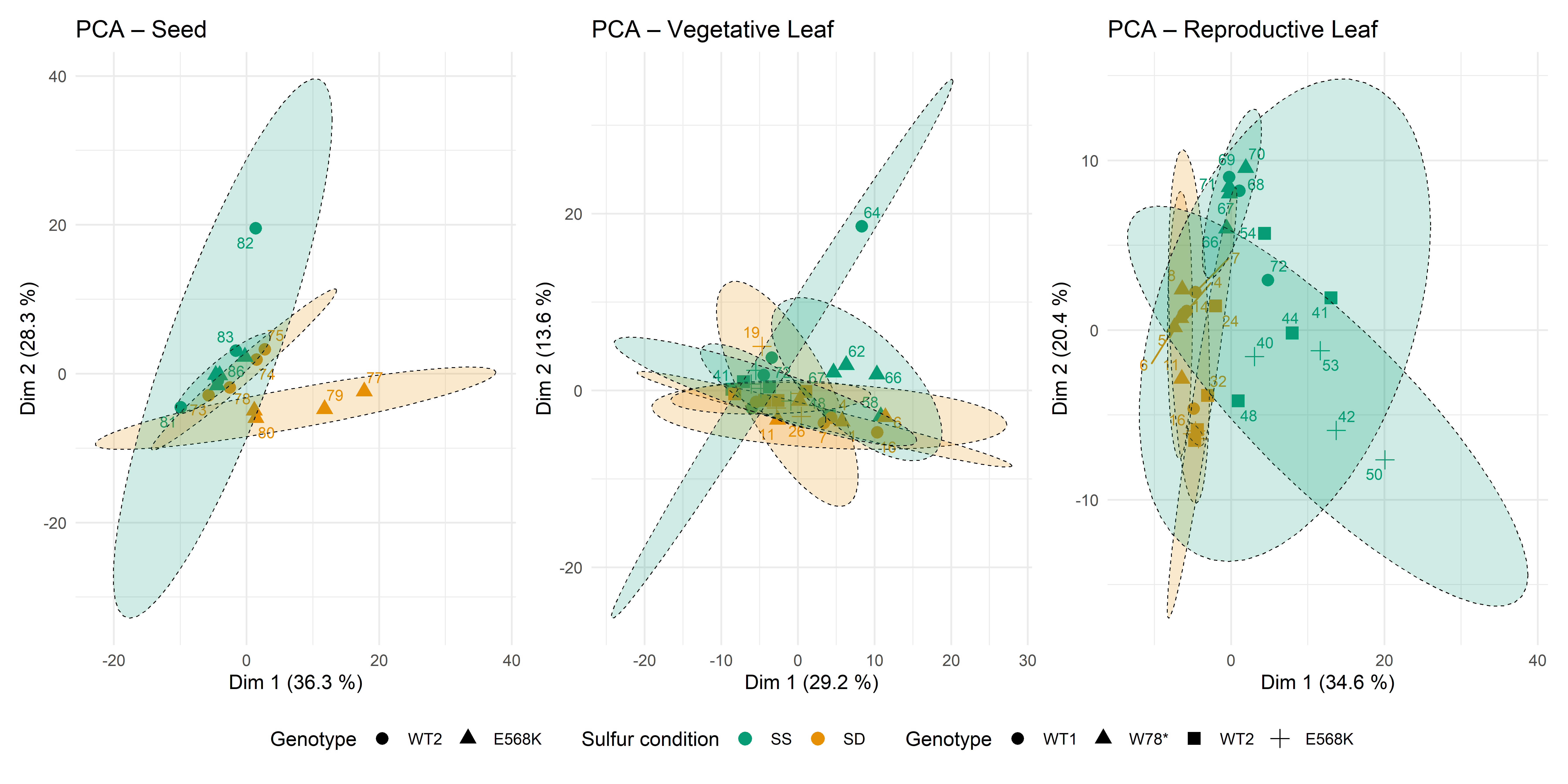 ### PLSDA ```{r, eval = F} df_metabo_global <- read_csv(here::here("data/metabolomic/output/df_metabolite_global_IBMP.csv"), show_col_types = FALSE) %>% mutate(sulfur_condition= fct_relevel(sulfur_condition, "SS", "SD"), genotype = fct_relevel(genotype, "WT1", "W78*", "WT2", "E568K"), type_genotype = fct_relevel(type_genotype, "WT", "Mut") )#%>% #filter(!str_detect(variable, "putative")) sulfate_palette <- c("SS" = as.character(sulfate_pallet[1]), "SD" = as.character(sulfate_pallet[2])) type_genotype_palette <- c("WT" = "#4f5bd5", "Mut" = "#d62976") # ── Helper that runs PLS-DA and returns a ggplot ────────────────────────── # ── Build the three plots ───────────────────────────────────────────────── group_i = "sulfur_condition" #group_i = "type_genotype" pal_i = sulfate_palette# type_genotype_palette p_seed <- plot_plsda_compartment(df_metabo_global, "seed", group_i = group_i, pal = pal_i) p_vleaf <- plot_plsda_compartment(df_metabo_global, "vegetative leaf", group_i = group_i, pal = pal_i) p_rleaf <- plot_plsda_compartment(df_metabo_global, "reproductive leaf", group_i = group_i, pal = pal_i) # ── Combine & export (optional) ─────────────────────────────────────────── combined_plsda <- (p_seed | p_vleaf | p_rleaf) + plot_layout(guides = "collect") & theme(legend.position = "bottom") # print to the graphics device combined_plsda # export # fig_export(here::here(paste0("report/metabolomic/plot/IBMP/PLSDA/without_putative",group_i)), combined_plsda, height_i = 6, width_i = 12, res_i = 600,format = "png") fig_export(here::here(paste0("report/metabolomic/plot/IBMP/PLSDA/with_putative",group_i)), combined_plsda, height_i = 6, width_i = 12, res_i = 600,format = "png") # For article # ── Helper that runs PLS-DA and returns a ggplot ────────────────────────── # ── Build the three plots ───────────────────────────────────────────────── group_i = "sulfur_condition" #group_i = "type_genotype" pal_i = sulfate_palette# type_genotype_palette p_vleaf <- plot_plsda_compartment(df_metabo_global, "vegetative leaf", group_i = group_i, pal = pal_i, show_id = F) + # légende sous le plot # theme(legend.position = "bottom") theme( legend.position = "bottom", # sous la figure legend.box = "vertical", # empile les guides verticalement legend.box.just = "left" # centre l’ensemble ) +labs(title = "", subtitle = "PLS-DA - Vegetative leaves - SS vs SD condition") p_vleaf # # ── Combine & export (optional) ─────────────────────────────────────────── # combined_plsda <- (p_vleaf | p_rleaf) + # plot_layout(guides = "collect") & # theme(legend.position = "bottom")& # plot_annotation( # tag_levels = 'A') # # # print to the graphics device # combined_plsda # export # fig_export(here::here(paste0("report/metabolomic/plot/IBMP/PLSDA/fig_x_without_putative_",group_i)), combined_plsda, height_i = 4, width_i = 7, res_i = 600) save(p_vleaf, file = here::here(paste0("report/metabolomic/plot/IBMP/PLSDA/fig_x_A_with_putative_",group_i, ".RData"))) ``` 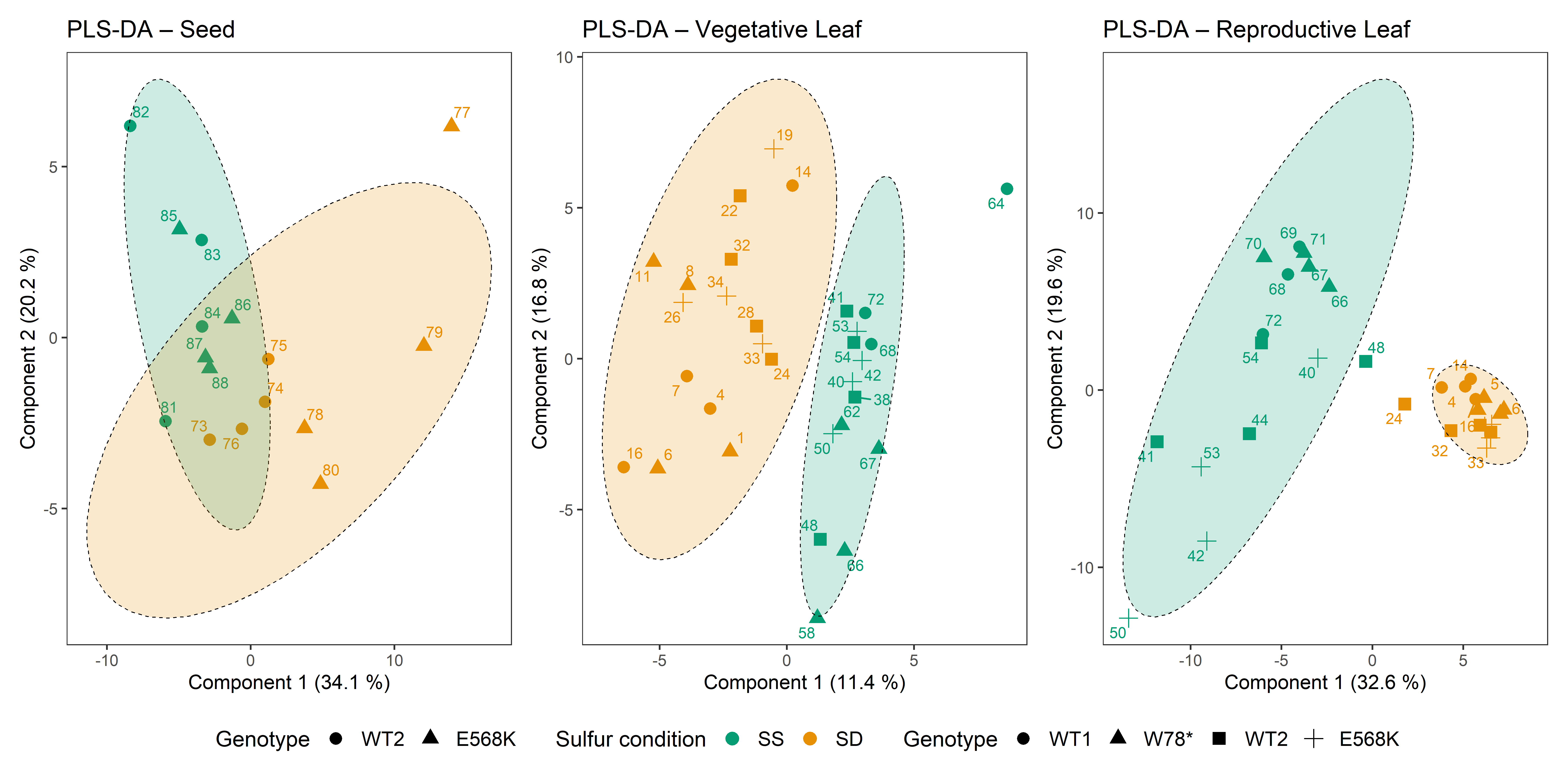 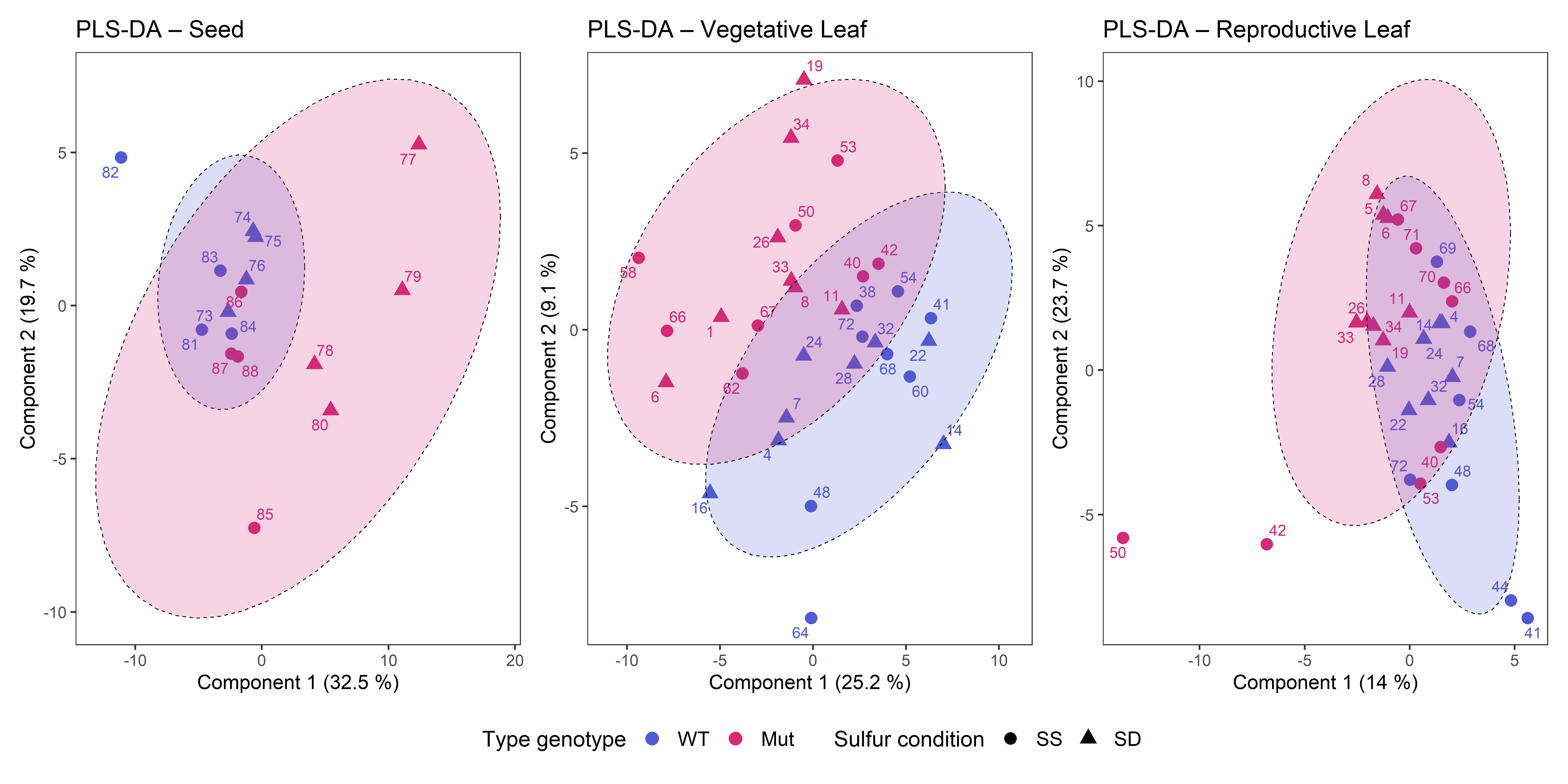  ```{r, eval = F} df_metabo_SS <- read_csv(here::here("data/metabolomic/output/df_metabolite_global_IBMP.csv"), show_col_types = FALSE) %>% mutate(sulfur_condition= fct_relevel(sulfur_condition, "SS", "SD"), genotype = fct_relevel(genotype, "WT1", "W78*", "WT2", "E568K"), type_genotype = fct_relevel(type_genotype, "WT", "Mut") ) %>% filter(sulfur_condition == "SS") # %>% # filter(!str_detect(variable, "putative")) df_metabo_SD <- read_csv(here::here("data/metabolomic/output/df_metabolite_global_IBMP.csv"), show_col_types = FALSE) %>% mutate(sulfur_condition= fct_relevel(sulfur_condition, "SS", "SD"), genotype = fct_relevel(genotype, "WT1", "W78*", "WT2", "E568K"), type_genotype = fct_relevel(type_genotype, "WT", "Mut") ) %>% filter(sulfur_condition == "SD") # %>% # filter(!str_detect(variable, "putative")) type_genotype_palette <- c("WT" = "#4f5bd5", "Mut" = "#d62976") # ── Helper that runs PLS-DA and returns a ggplot ────────────────────────── # ── Build the three plots ───────────────────────────────────────────────── group_i = "type_genotype" #group_i = "type_genotype" pal_i = type_genotype_palette # type_genotype_palette p_seed <- plot_plsda_compartment(df_metabo_SD, "seed", group_i = group_i, pal = pal_i) p_vleaf <- plot_plsda_compartment(df_metabo_SD, comp = "vegetative leaf", group_i = group_i, pal = pal_i) p_rleaf <- plot_plsda_compartment(df_metabo_SD, "reproductive leaf", group_i = group_i, pal = pal_i) # ── Combine & export (optional) ─────────────────────────────────────────── combined_plsda <- (p_seed | p_vleaf | p_rleaf) + plot_layout(guides = "collect") & theme(legend.position = "bottom") # print to the graphics device combined_plsda # export fig_export(here::here(paste0("report/metabolomic/plot/IBMP/PLSDA/SD_without_putative",group_i)), combined_plsda, height_i = 6, width_i = 12, res_i = 600,format = "png") ###############for article p_vleaf_SS <- plot_plsda_compartment(df_metabo_SS, comp = "vegetative leaf", group_i = group_i, pal = pal_i)+labs(title = "", subtitle = "PLS-DA - Vegetative leaves - SS condition") p_vleaf_SD <- plot_plsda_compartment(df_metabo_SD, comp = "vegetative leaf", group_i = group_i, pal = pal_i)+labs(title = "", subtitle = "PLS-DA - Vegetative leaves - SD condition") # p_rleaf <- plot_plsda_compartment(df_metabo_SD, "reproductive leaf", group_i = group_i, pal = pal_i) # ── Combine & export (optional) ─────────────────────────────────────────── # combined_plsda <- (p_vleaf | p_rleaf) + # plot_layout(guides = "collect") & # theme(legend.position = "bottom")& # plot_annotation( # tag_levels = 'A') # # # print to the graphics device # combined_plsda # export # fig_export(here::here(paste0("report/metabolomic/plot/IBMP/PLSDA/Fig_X_SD_without_putative_",group_i)), combined_plsda, height_i = 4, width_i = 7, res_i = 600) save(p_vleaf_SD, p_vleaf_SS, file = here::here(paste0("report/metabolomic/plot/IBMP/PLSDA/fig_x_CE_with_putative_type_genotype.RData"))) ``` 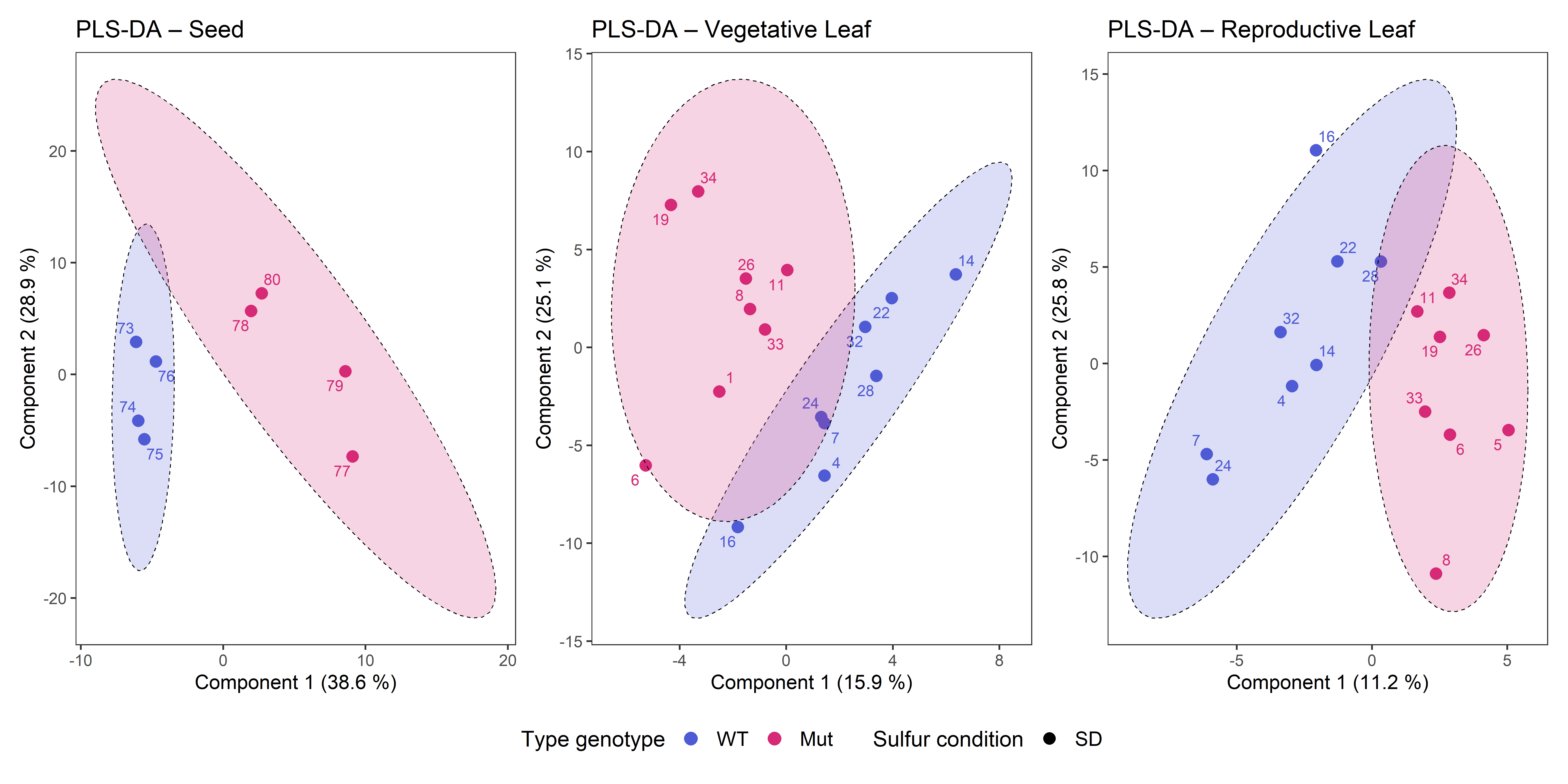 ```{r, eval = F} # data df_metabo_global <- read_csv(here::here("data/metabolomic/output/df_metabolite_global_IBMP.csv"), show_col_types = FALSE) %>% mutate(sulfur_condition= fct_relevel(sulfur_condition, "SS", "SD"), genotype = fct_relevel(genotype, "WT1", "W78*", "WT2", "E568K"), type_genotype = fct_relevel(type_genotype, "WT", "Mut") )%>% filter(!str_detect(variable, "putative")) # function plot_plsda_loadings <- function(data, comp = "seed", # compartment group_i = "sulfur_condition", ncomp = 5, # total comps in model method = "mean", # how to average contrib = "max", # highlight criterion component_i = 1, ndisplay = 30) { # top variables to show # 1. reshape & average duplicates --------------------------------------- df_wide <- data %>% filter(compartment == comp) %>% dplyr::select(plant_num, genotype, type_genotype, sulfur_condition, condition, variable, value) %>% pivot_wider(names_from = variable, values_from = value) %>% mutate(plant_num = as.factor(plant_num)) %>% dplyr::group_by(plant_num, genotype, type_genotype, sulfur_condition, condition) %>% dplyr::summarise(across(where(is.numeric), mean, na.rm = TRUE), .groups = "drop") # 2. build X (predictors) & Y (class) ------------------------------------ X <- df_wide %>% dplyr::select(where(is.numeric)) %>% dplyr::select(where(~ sd(.) != 0)) %>% # drop zero-variance cols as.matrix() Y <- factor(df_wide[[group_i]]) # 3. PLS-DA -------------------------------------------------------------- mod <- plsda(X, Y, ncomp = ncomp) # 4. Loadings plot for components 1 & 2 ---------------------------------- p <- plotLoadings(mod, comp = component_i, method = method, contrib = contrib, ndisplay = ndisplay, title = paste("PLS-DA loadings ",str_to_title_clean(comp), "\n", "Component ", component_i,".", str_to_title_clean(group_i), " effect"), size.title = rel(1), style = "ggplot") # returns a ggplot object } comp_i = "seed" group_i = "sulfur_condition" component_i = 1 params <- expand.grid( comp_i = c("seed", "vegetative leaf", "reproductive leaf"), group_i = c("genotype", "type_genotype", "sulfur_condition"), component_i = c(1, 2), stringsAsFactors = FALSE ) for (i in 1:nrow(params)){ # param comp_i = params$comp_i[i] group_i = params$group_i[i] component_i = params$component_i[i] svg(width = 10, height = 5, here::here(paste0("report/metabolomic/plot/IBMP/plotLoadings/without_putative", str_to_title_clean(group_i), "_",str_to_title_clean(comp_i), "_", component_i, ".svg"))) load_seed1 <- plot_plsda_loadings(df_metabo_global, comp_i, group_i = group_i, component_i = component_i, ndisplay = 15) dev.off() } # in SD condition only # data df_metabo_SD <- read_csv(here::here("data/metabolomic/output/df_metabolite_global_IBMP.csv"), show_col_types = FALSE) %>% mutate(sulfur_condition= fct_relevel(sulfur_condition, "SS", "SD"), genotype = fct_relevel(genotype, "WT1", "W78*", "WT2", "E568K"), type_genotype = fct_relevel(type_genotype, "WT", "Mut") ) %>% filter(sulfur_condition == "SD") %>% filter(!str_detect(variable, "putative")) params <- expand.grid( comp_i = c("seed", "vegetative leaf", "reproductive leaf"), group_i = c("genotype", "type_genotype"), component_i = c(1, 2), stringsAsFactors = FALSE ) for (i in 1:nrow(params)){ # param comp_i = params$comp_i[i] group_i = params$group_i[i] component_i = params$component_i[i] svg(width = 10, height = 5, here::here(paste0("report/metabolomic/plot/IBMP/plotLoadings/SD_without_putative", str_to_title_clean(group_i), "_",str_to_title_clean(comp_i), "_", component_i, ".svg"))) load_seed1 <- plot_plsda_loadings(df_metabo_SD, comp_i, group_i = group_i, component_i = component_i, ndisplay = 15) dev.off() } ``` ```{r, echo=FALSE, results = "asis"} # function remove_terms <- function(text_vec, terms_vec, ignore_case = TRUE) { # Construit une regex du type "\\b(terme1|terme2|terme3)\\b" pattern <- paste0("\\b(", paste(terms_vec, collapse = "|"), ")\\b") text_vec %>% str_remove_all(regex(pattern, ignore_case = ignore_case)) %>% str_squish() # retire les espaces multiples laissés par la suppression } word_to_del <- c("Genotype", "Reproductive leaf_", "Vegetative leaf_", "Sulfur condition_", "Type genotype_") image_files <- list.files("plot/IBMP/plotLoadings", pattern = "\\.svg$", full.names = TRUE) # Extraire le nom des fichiers sans extension image_names <- tools::file_path_sans_ext(basename(image_files)) # Extraire la première et la deuxième valeur séparées par "_" first_values <- sapply(strsplit(image_names, "_"), function(x) x[1]) second_values <- sapply(strsplit(image_names, "_"), function(x) x[2]) # Identifier les groupes uniques pour la première valeur unique_first <- unique(first_values) # Création du code pour le panel-tabset global tabset_code <- ":::: {.panel-tabset}\n" # Pour chaque groupe du premier niveau for (grp1 in unique_first) { tabset_code <- paste0(tabset_code, "## ", grp1, "\n\n", ":::: {.panel-tabset}\n") # Indices des images appartenant à ce groupe indices_first <- which(first_values == grp1) # Identifier les sous-groupes (deuxième valeur) dans ce groupe unique_second <- unique(second_values[indices_first]) # Pour chaque sous-groupe du deuxième niveau for (grp2 in unique_second) { tabset_code <- paste0(tabset_code, "### ", grp2, "\n\n", ":::: {.panel-tabset}\n") # Sélectionner les images correspondant à ce sous-groupe indices_second <- indices_first[second_values[indices_first] == grp2] for (i in indices_second) { tabset_code <- paste0(tabset_code, "#### ", remove_terms(image_names[i], word_to_del), "\n\n", " } tabset_code <- paste0(tabset_code, "::::\n\n") # fermeture du sous-tabset du deuxième niveau } tabset_code <- paste0(tabset_code, "::::\n\n") # fermeture du sous-tabset du premier niveau } tabset_code <- paste0(tabset_code, "::::") cat(tabset_code) ``` ### Show the graphs with the stats for the strongest loading ```{r, eval = F} df_metabo_global <- read_csv(here::here("data/metabolomic/output/df_metabolite_global_IBMP.csv"), show_col_types = FALSE) %>% mutate(sulfur_condition= fct_relevel(sulfur_condition, "SS", "SD"), genotype = fct_relevel(genotype, "WT1", "W78*", "WT2", "E568K"), type_genotype = fct_relevel(type_genotype, "WT", "Mut") ) all_possibility <- df_metabo_global %>% distinct(variable,compartment) # Initialisation de la liste qui va stocker tous les plots plots <- list() # Boucle sur chaque combinaison for (i in seq_len(nrow(all_possibility))) { variable_i <- all_possibility$variable[i] compartment_i <- all_possibility$compartment[i] # Filtrage des données pour la combinaison courante df_select <- df_metabo_global %>% filter( variable == variable_i, compartment == compartment_i ) %>% drop_na(value) %>% as.data.frame() # Si aucune donnée n'est disponible, on passe à la combinaison suivante if(nrow(df_select) == 0) { message("Aucune donnée pour: ", stage_i, ", ", element_i, ", ", compartment_i) next } # Définition de l'étiquette de l'axe des ordonnées ylab_i <- paste0(str_to_title_clean(variable_i), " in ", compartment_i) # Essayer d'exécuter stat_analyse et capturer les erreurs éventuelles res <- tryCatch({ stat_analyse( data = df_select, column_value = "value", category_variables = c("sulfur_condition"), grp_var = "genotype", show_plot = TRUE, outlier_show = FALSE, label_outlier = "plant_num", biologist_stats = TRUE, Ylab_i = ylab_i, control_conditions = c("SS"), strip_normale = FALSE, hex_pallet = sulfate_pallet ) }, error = function(e) { message("Erreur pour: ", ", ", variable_i, ", ", compartment_i, " -> ", e$message) return(NULL) }) # Si une erreur s'est produite, on passe à l'itération suivante if(is.null(res)) next # Extraction du plot et ajout des labels pour la légende p_plot <- res[["plot"]] + labs(color = "Treatment", fill = "Treatment") plot_name <- paste0(compartment_i, "_", str_to_title_clean(variable_i)) fig_export(here::here(paste0("report/metabolomic/plot/IBMP/plot_stats/", plot_name)), p_plot, height_i = 4, width_i = 5, res_i = 300,format = "png") plots[[plot_name]] <- p_plot } # # Assemblage de tous les plots avec patchwork # final_plot <- wrap_plots(plots, ncol = 6) + # plot_layout(guides = "collect") + # plot_annotation() & theme(legend.position = 'bottom') # # # Affichage du plot final # print(final_plot) # fig_export(here::here("report/CNS/plot/all_CNS_stats"), final_plot, height_i = 21, width_i = 29.7, res_i = 600) ``` ```{r, echo=FALSE, results = "asis"} # function remove_terms <- function(text_vec, terms_vec, ignore_case = TRUE) { # Construit une regex du type "\\b(terme1|terme2|terme3)\\b" pattern <- paste0("\\b(", paste(terms_vec, collapse = "|"), ")\\b") text_vec %>% str_remove_all(regex(pattern, ignore_case = ignore_case)) %>% str_squish() # retire les espaces multiples laissés par la suppression } word_to_del <- c("seed_", "reproductive leaf_", "vegetative leaf_") image_files <- list.files("plot/IBMP/plot_stats/", pattern = "\\.png$", full.names = TRUE) # Extraire le nom des fichiers sans extension image_names <- tools::file_path_sans_ext(basename(image_files)) # Extraire la première et la deuxième valeur séparées par "_" first_values <- sapply(strsplit(image_names, "_"), function(x) x[1]) second_values <- sapply(strsplit(image_names, "_"), function(x) x[2]) # Identifier les groupes uniques pour la première valeur unique_first <- unique(first_values) # Création du code pour le panel-tabset global tabset_code <- ":::: {.panel-tabset}\n" # Pour chaque groupe du premier niveau for (grp1 in unique_first) { tabset_code <- paste0(tabset_code, "## ", grp1, "\n\n", ":::: {.panel-tabset}\n") # Indices des images appartenant à ce groupe indices_first <- which(first_values == grp1) # Identifier les sous-groupes (deuxième valeur) dans ce groupe unique_second <- unique(second_values[indices_first]) # Pour chaque sous-groupe du deuxième niveau for (grp2 in unique_second) { tabset_code <- paste0(tabset_code, "### ", grp2, "\n\n", ":::: {.panel-tabset}\n") # Sélectionner les images correspondant à ce sous-groupe indices_second <- indices_first[second_values[indices_first] == grp2] for (i in indices_second) { tabset_code <- paste0(tabset_code, "#### ", remove_terms(image_names[i], word_to_del), "\n\n", " } tabset_code <- paste0(tabset_code, "::::\n\n") # fermeture du sous-tabset du deuxième niveau } tabset_code <- paste0(tabset_code, "::::\n\n") # fermeture du sous-tabset du premier niveau } tabset_code <- paste0(tabset_code, "::::") cat(tabset_code) ``` ```{r, eval = F} #test to see some boxpltot # data df_metabo_global <- read_csv(here::here("data/metabolomic/output/df_metabolite_global_IBMP.csv"), show_col_types = FALSE) %>% mutate(sulfur_condition= fct_relevel(sulfur_condition, "SS", "SD"), genotype = fct_relevel(genotype, "WT1", "W78*", "WT2", "E568K"), type_genotype = fct_relevel(type_genotype, "WT", "Mut") )%>% filter(!str_detect(variable, "putative")) %>% filter(sulfur_condition == "SD") levels(as.factor(df_metabo_global$variable)) compound_i <- "Compound 22: glutamic acid" compound_i <- "phenylalanine" compound_i <- "tartric acid" compound_i <- "Compound 57: melibiose" compound_i <- "glyceric acid" df_select<- df_metabo_global %>% filter(compartment == "vegetative leaf", variable == compound_i ) %>% as.data.frame() type_genotype_palette <- c("WT" = "#4f5bd5", "Mut" = "#d62976") stat_analyse( data = df_select, column_value = "value", category_variables = c("type_genotype"), grp_var = "genotype", show_plot = TRUE, outlier_show = FALSE, label_outlier = "plant_num", biologist_stats = TRUE, Ylab_i = compound_i, control_conditions = c("SS"), strip_normale = FALSE, hex_pallet = type_genotype_palette ) ``` ### VIP ```{r, eval = F} #data importation df_metabo_global <- read_csv(here::here("data/metabolomic/output/df_metabolite_global_IBMP.csv"), show_col_types = FALSE) %>% mutate(sulfur_condition= fct_relevel(sulfur_condition, "SS", "SD"), genotype = fct_relevel(genotype, "WT1", "W78*", "WT2", "E568K"), type_genotype = fct_relevel(type_genotype, "WT", "Mut") )#%>% #filter(!str_detect(variable, "putative")) # function plot_VIP <- function(data, comp = "vegetative leaf", group_i = "sulfur_condition", ncomp = 5, component_i = 1, ndisplay = 30) { library(dplyr); library(tidyr); library(forcats); library(ggplot2); library(mixOmics) ## 1. Sous-ensemble du compartiment --------------------------------- long_comp <- data %>% filter(compartment == comp) %>% mutate(group_select = .data[[group_i]]) ## 2. Moyennes SD vs SS pour la coloration --------------------------- mean_cond <- long_comp %>% # long format group_by(variable, group_select) %>% summarise(mean_val = mean(value, na.rm = TRUE), .groups = "drop") %>% pivot_wider(names_from = group_select, values_from = mean_val) lvls <- setdiff(names(mean_cond), "variable") # mean_cond = mean_cond %>% # mutate(direction = ifelse(SD > SS, "SD higher", "SD lower"), # fill_col = ifelse(direction == "SD higher","#ee3e32", "#1d4877" )) %>% # dplyr::select(variable, direction, fill_col) grp_cols <- setdiff(names(mean_cond), "variable") # ex. c("control", "stress") stopifnot(length(grp_cols) == 2) # sécurité cols <- c(control = "#1d4877", # adapte une seule fois stress = "#ee3e32", WT = "#1d4877", Mut = "#ee3e32", SS = "#1d4877", SD = "#ee3e32") mean_cond <- mean_cond %>% rowwise() %>% # traiter ligne par ligne mutate( direction = paste0( grp_cols[ which.max(c_across(all_of(grp_cols))) ], " higher" ), fill_col = cols[ sub(" higher$", "", direction) ] # couleur gagnante ) %>% ungroup() %>% select(variable, direction, fill_col) ## 3. Construction du jeu large & modèle PLS-DA ---------------------- df_wide <- long_comp %>% dplyr::select(plant_num, genotype, type_genotype, sulfur_condition, condition, variable, value) %>% pivot_wider(names_from = variable, values_from = value) %>% mutate(plant_num = as.factor(plant_num)) %>% dplyr::group_by(plant_num, genotype, type_genotype, sulfur_condition, condition) %>% dplyr::summarise(across(where(is.numeric), mean, na.rm = TRUE), .groups = "drop") X <- df_wide %>% select(where(is.numeric)) %>% select(where(~ sd(.) != 0)) %>% as.matrix() Y <- factor(df_wide[[group_i]]) mod <- plsda(X, Y, ncomp = ncomp) vip_c <- vip(mod)[ , component_i] # VIP de la composante voulue ## 4. Préparation des données pour le barplot ------------------------ vip_df <- tibble(variable = names(vip_c), VIP = as.numeric(vip_c)) %>% arrange(desc(VIP)) %>% slice_head(n = ndisplay) %>% # top N left_join(mean_cond, by = "variable") %>% # ajoute couleurs mutate( fill_col = replace_na(fill_col, "grey80"), # si SD ou SS manquant variable = fct_reorder(variable, VIP), VIP_label = sprintf("%.2f", VIP) ) ## 5. Barplot horizontal -------------------------------------------- ggplot(vip_df, aes(x = VIP, y = variable, fill = fill_col)) + geom_col() + geom_text(aes(label = VIP_label), hjust = -0.1, size = 3) + geom_vline(xintercept = 1, linetype = "dashed") + scale_fill_identity(guide = "legend", breaks = c("#ee3e32", "#1d4877"), labels = c(paste0(lvls[2]," > ", lvls[1]), paste0(lvls[2]," < ", lvls[1])), name = "Direction") + scale_x_continuous(expand = expansion(mult = c(0, 0.15))) + labs(#title = "Variable Importance in Projection (VIP)", subtitle = sprintf("Component %i – %s", component_i, comp), x = "VIP value", y = NULL) + theme_bw() + theme(axis.text.y = element_text(size = 8), plot.title = element_text(face = "bold")) } group_i = "sulfur_condition" p_vl_sulfur_condition <- plot_VIP(df_metabo_global,comp = "vegetative leaf", # "vegetative leaf", # compartment group_i = "sulfur_condition", ncomp = 3, # total comps in model component_i = 1, ndisplay = 30)+ labs(subtitle = "Component 1 - Vegetative leaves SS vs SD") # p_rl <- plot_VIP(df_metabo_global,comp = "reproductive leaf", # "vegetative leaf", # compartment # group_i = "sulfur_condition", # ncomp = 3, # total comps in model # component_i = 1, # ndisplay = 30) # combined_VIP_sulfur_condition <- (p_vl | p_rl) + # plot_layout(guides = "collect") & # theme(legend.position = "bottom")& # plot_annotation( # tag_levels = 'A', # title = "VIP scores for Component 1 of the PLS-DA model", # theme = theme( # plot.title = element_text(size = 14, face = "bold", hjust = 0.1) # ) # ) # print to the graphics device # combined_VIP_sulfur_condition # group_i = "type_genotype" # export # fig_export(here::here(paste0("report/metabolomic/plot/IBMP/VIP/All_with_putative_",group_i)), combined_VIP_sulfur_condition, height_i = 8, width_i = 12, res_i = 600) save(p_vl_sulfur_condition, file = here::here(paste0("report/metabolomic/plot/IBMP/VIP/fig_x_B_with_putative_",group_i, ".RData"))) # for SD only for mutant familly ############################################### df_metabo_global_ss <- read_csv(here::here("data/metabolomic/output/df_metabolite_global_IBMP.csv"), show_col_types = FALSE) %>% mutate(sulfur_condition= fct_relevel(sulfur_condition, "SS", "SD"), genotype = fct_relevel(genotype, "WT1", "W78*", "WT2", "E568K"), type_genotype = fct_relevel(type_genotype, "WT", "Mut") )%>% #filter(!str_detect(variable, "putative")) %>% filter(sulfur_condition == "SS") df_metabo_global_sd <- read_csv(here::here("data/metabolomic/output/df_metabolite_global_IBMP.csv"), show_col_types = FALSE) %>% mutate(sulfur_condition= fct_relevel(sulfur_condition, "SS", "SD"), genotype = fct_relevel(genotype, "WT1", "W78*", "WT2", "E568K"), type_genotype = fct_relevel(type_genotype, "WT", "Mut") )%>% #filter(!str_detect(variable, "putative")) %>% filter(sulfur_condition == "SD") p_vl_ss_VIP <- plot_VIP(df_metabo_global_ss, comp = "vegetative leaf", # "vegetative leaf", # compartment group_i = "type_genotype", ncomp = 3, # total comps in model component_i = 1, ndisplay = 30)+ labs(subtitle = "Component 1 - Vegetative leaves - WT vs Mut - SS") p_vl_sd_VIP <- plot_VIP(df_metabo_global_sd, comp = "vegetative leaf", # "vegetative leaf", # compartment group_i = "type_genotype", ncomp = 3, # total comps in model component_i = 1, ndisplay = 30)+ labs(subtitle = "Component 1 - Vegetative leaves - WT vs Mut - SD") # p_rl_sd <- plot_VIP(df_metabo_global_sd, # comp = "reproductive leaf", # "vegetative leaf", # compartment # group_i = "type_genotype", # ncomp = 3, # total comps in model # component_i = 1, # ndisplay = 30) save(p_vl_ss_VIP, p_vl_sd_VIP, file = here::here(paste0("report/metabolomic/plot/IBMP/VIP/fig_x_DF_with_putative_type_genotype.RData"))) # combined_VIP_sd_mutant_type <- (p_vl_sd | p_rl_sd) + # plot_layout(guides = "collect") & # theme(legend.position = "bottom")& # plot_annotation( # tag_levels = 'A', # title = "VIP scores for Component 1 of the PLS-DA model", # theme = theme( # plot.title = element_text(size = 14, face = "bold", hjust = 0.1) # ) # ) # print to the graphics device # combined_VIP_sd_mutant_type # export # fig_export(here::here(paste0("report/metabolomic/plot/IBMP/VIP/SD_with_putative_",group_i)), combined_VIP_sd_mutant_type, height_i = 8, width_i = 12, res_i = 600) ``` ```{r, eval = F} load(file = here::here(paste0("report/metabolomic/plot/IBMP/PLSDA/fig_x_A_with_putative_sulfur_condition.RData"))) # p_vleaf load(file = here::here(paste0("report/metabolomic/plot/IBMP/VIP/fig_x_B_with_putative_sulfur_condition.RData"))) # p_vl_sulfur_condition load(file = here::here(paste0("report/metabolomic/plot/IBMP/PLSDA/fig_x_CE_with_putative_type_genotype.RData"))) # p_vleaf_SD, p_vleaf_SS load(file = here::here(paste0("report/metabolomic/plot/IBMP/VIP/fig_x_DF_with_putative_type_genotype.RData"))) # p_vl_ss_VIP, p_vl_sd_VIP #combine plot combined_AB <- (p_vleaf | p_vl_sulfur_condition) + plot_layout(guides = "collect") & theme(legend.position = "right")& plot_annotation( tag_levels = 'A', # title = "VIP scores for Component 1 of the PLS-DA model", theme = theme( plot.title = element_text(size = 14, face = "bold", hjust = 0.1) ) ) combined_CDEF <- (p_vleaf_SS + guides(shape = "none")|p_vl_ss_VIP ) / (p_vleaf_SD + guides(shape = "none")| p_vl_sd_VIP)+ plot_layout(guides = "collect") & theme(legend.position = "right")& plot_annotation( tag_levels = 'A', # title = "VIP scores for Component 1 of the PLS-DA model", theme = theme( plot.title = element_text(size = 14, face = "bold", hjust = 0.1) ) ) combined_fig_X <- combined_AB/combined_CDEF+ plot_layout(heights = c(1, 2.5)) & plot_annotation( tag_levels = 'A', # title = "VIP scores for Component 1 of the PLS-DA model", theme = theme( plot.title = element_text(size = 14, face = "bold", hjust = 0.1) ) ) fig_export(here::here(paste0("report/metabolomic/plot/IBMP/Fig_X_with_putative")), combined_fig_X, height_i = 15, width_i = 12, res_i = 600) ```  ### Heatmap for vegetative and reproductive leaves ```{r, eval = F} df_metabo_global <- read_csv(here::here("data/metabolomic/output/df_metabolite_global_IBMP.csv"), show_col_types = FALSE) %>% mutate(sulfur_condition= fct_relevel(sulfur_condition, "SS", "SD"), genotype = fct_relevel(genotype, "WT1", "W78*", "WT2", "E568K"), type_genotype = fct_relevel(type_genotype, "WT", "Mut") ) # data importation df_metabo_select <- df_metabo_global %>% filter(compartment == "vegetative leaf") %>% mutate(comp_metabo = paste0(compartment, "_", variable)) %>% dplyr::select(plant_num, genotype, sulfur_condition,comp_metabo, value) df_metabo_select_h <- df_metabo_select %>% pivot_wider(names_from = comp_metabo, values_from = value) variable <- colnames(df_metabo_select_h[4:length(df_metabo_select_h)]) matrix_scale_select <- df_metabo_select_h %>% dplyr::select(plant_num, all_of(variable)) %>% { cols_to_keep <- sapply(.[, -1], function(x) !(is.numeric(x) && var(x, na.rm = TRUE) == 0)) dplyr::select(., plant_num, names(cols_to_keep)[cols_to_keep]) } %>% column_to_rownames("plant_num") %>% as.matrix() matrix_standardized <- scale(matrix_scale_select, center = TRUE, scale = TRUE) # modifier pour avoir des variables uniquement entre 0 et 1 normalize_min_max <- function(x) { (x - min(x, na.rm = TRUE)) / (max(x, na.rm = TRUE) - min(x, na.rm = TRUE)) * 2 - 1 } matrix_standardized<-as.data.frame (matrix_scale_select) %>% dplyr::mutate(across(everything(), normalize_min_max)) ###### # Finding the optimal number of clusters (begin) ####### hc.cols <- hclust(dist(t(matrix_standardized)), method = "ward.D2") hc.cols <- hclust(dist(t(matrix_standardized), method = "euclidean"), method = "complete") plot(hc.cols, sub = "", xlab = "", main = "Clusters des paramètres") # Calculate distance matrix distance_matrix <- dist(t(matrix_standardized)) # fviz_nbclust(as.data.frame(distance_matrix), FUN = hcut, method = "wss") # fviz_nbclust(as.data.frame(distance_matrix), FUN = hcut, method = "silhouette") # fviz_nbclust(as.data.frame(distance_matrix), FUN = hcut, method = "gap_stat", nboot = 50) # Select a random subset of columns set.seed(100) # For the reproductibility sample_columns <- sample(ncol(matrix_standardized), 40) matrix_sample <- matrix_standardized[, sample_columns] # Calculate the distance matrix on the subset distance_matrix_sample <- dist(t(matrix_sample)) # Use fviz_nbclust for the subset fviz_nbclust(as.data.frame(distance_matrix_sample), FUN = hcut, method = "wss", k.max = 20) fviz_nbclust(as.data.frame(distance_matrix_sample),FUN = hcut, method = "silhouette", k.max = 20) fviz_nbclust(as.data.frame(distance_matrix_sample),FUN = hcut, method = "gap_stat", k.max = 20) # or with PCA # Dimension reduction with PCA (keeping the first 20 components) pca_result <- prcomp(matrix_standardized, center = TRUE, scale. = TRUE) matrix_reduced <- pca_result$x[, 1:32] # Calculate distance matrix for principal components distance_matrix_pca <- dist(matrix_reduced) # Use fviz_nbclust to determine the number of clusters fviz_nbclust(as.data.frame(distance_matrix_pca), FUN = hcut, method = "wss") ###### # Finding the optimal number of clusters (end) ####### # parameter num_clusters <- 5 # Number of cluster cluster_assignments <- cutree(hc.cols, k = num_clusters) # Associate each variable with its cluster clustered_variables <- data.frame( variable = colnames(matrix_standardized), cluster = cluster_assignments ) annotation_row <- df_metabo_select_h %>% distinct(plant_num, genotype, sulfur_condition) %>% column_to_rownames("plant_num") %>% dplyr::rename(Genotype = genotype, `Sulfur condition`= sulfur_condition ) ################## annotation_col <- data.frame(variable = colnames(matrix_standardized)) %>% full_join(., clustered_variables, by="variable") %>% mutate(cluster = as.character(cluster)) %>% column_to_rownames("variable") %>% dplyr::rename(Cluster = cluster)# rename col cluster to be the same as annotation_colors # levels(as.factor(annotation_col$variable_type)) my_color_palette <- read_excel(here::here("data/color_palette.xlsm")) color_cluster_v=c(my_color_palette %>% filter(set=="cluster") %>% pull(color), "gray20", "gray70" ) # palette <- colorRampPalette(c("#01a2a4", "#FFD275", "#e3420e"))(500) palette <- viridis::viridis(500) annotation_colors <- list( `Sulfur condition` = c(sulfate_pallet), Genotype = mutant_palette, Cluster = setNames(color_cluster_v[1:11], as.character(1:11)) ) #heatmap(matrix_standardized,Colv=T, scale='none', col=palette,cexCol=0.6) heatmap_all <- pheatmap(matrix_standardized, scale = "none", cluster_rows = T, cluster_cols = TRUE, #main = paste("Heatmap global"), color = palette, annotation_col = annotation_col, annotation_row = annotation_row, annotation_colors = annotation_colors, cutree_cols = num_clusters, show_rownames = T, show_colnames = F #cex = 0.8 ) ; heatmap_all # export fig_export(path = "report/metabolomic/plot/IBMP/heatmap/heatmap_vegetative", plot_x = heatmap_all, height_i = 9, width_i = 18, res = 600) ```  ## Venn diagram ## Nothing significant with BH correction... except SS vs SD in the reproductive parts... ```{r, eval = F} # data importation df_metabo_select <- read_csv(here::here("data/metabolomic/output/df_metabolite_global_IBMP.csv"), show_col_types = FALSE) %>% mutate(sulfur_condition= fct_relevel(sulfur_condition, "SS", "SD"), genotype = fct_relevel(genotype, "WT1", "W78*", "WT2", "E568K"), type_genotype = fct_relevel(type_genotype, "WT", "Mut") ) %>% #filter(compartment == "reproductive leaf") filter(compartment == "vegetative leaf") # i need a list for metabolite source(here::here("src/function/log_fc_pval.R")) # Function for calculate log, pval SS_WT_vs_SD_WT<- log_fc_pval(df_input = df_metabo_select %>% filter(genotype %in% c("WT1", "WT2")), # filter if needed type_condition = "sulfur_condition", controle_i = "SS", treatment_i = "SD" ) ; head(SS_WT_vs_SD_WT) # for each family ##For SS `WT_SS_WT1 vs Mut_SS_W78*` <- log_fc_pval(df_input = df_metabo_select %>% filter(sulfur_condition == "SS", genotype %in% c("WT1", "W78*")) , #%>% filter(genotype %in% c("WT1", "WT2")), # filter if needed type_condition = "type_genotype", controle_i = "WT", treatment_i = "Mut" ) ; head(`WT_SS_WT1 vs Mut_SS_W78*`) `WT_SS_WT2 vs Mut_SS_E568K` <- log_fc_pval(df_input = df_metabo_select %>% filter(sulfur_condition == "SS", genotype %in% c("WT2", "E568K")) , #%>% filter(genotype %in% c("WT1", "WT2")), # filter if needed type_condition = "type_genotype", controle_i = "WT", treatment_i = "Mut" ) ; head(`WT_SS_WT2 vs Mut_SS_E568K`) ## For SD `WT_SD_WT1 vs Mut_SD_W78*` <- log_fc_pval(df_input = df_metabo_select %>% filter(sulfur_condition == "SD", genotype %in% c("WT1", "W78*")) , #%>% filter(genotype %in% c("WT1", "WT2")), # filter if needed type_condition = "type_genotype", controle_i = "WT", treatment_i = "Mut" ) ; head(`WT_SD_WT1 vs Mut_SD_W78*`) `WT_SD_WT2 vs Mut_SD_E568K` <- log_fc_pval(df_input = df_metabo_select %>% filter(sulfur_condition == "SD", genotype %in% c("WT2", "E568K")) , #%>% filter(genotype %in% c("WT1", "WT2")), # filter if needed type_condition = "type_genotype", controle_i = "WT", treatment_i = "Mut" ) ; head(`WT_SD_WT2 vs Mut_SD_E568K`) Mutant_vs_WT_SD <- log_fc_pval(df_input = df_metabo_select %>% filter(sulfur_condition == "SD"), #%>% filter(genotype %in% c("WT1", "WT2")), # filter if needed type_condition = "type_genotype", controle_i = "WT", treatment_i = "Mut" ) ; head(Mutant_vs_WT_SD) ################# # get_genes<- function(df_comparison_i, lfc_lim = lfc_lim_i, padj_lim= 0.05, sign_i){ # change value here to change parameter # v_gene = df_comparison_i %>% # mutate(sign= ifelse(logFC>0, "Up", "Down")) %>% # filter( # sign == sign_i, # abs(logFC)>abs(lfc_lim), # PValue_standard<= padj_lim # !!!!!!!!!!!!!!!!!!!!!!!!!!!!!!!!!!!!!!!!!!!!!!!!!!!!!! # ) %>% # pull(variable) # return(v_gene) # } # # lfc_lim_i = 0 # padj_lim = 0.05 # # get_genes(df_comparison_i = SS_WT_vs_SD_WT, sign_i = "Up",lfc_lim = lfc_lim_i) # # lt_up_simplified <- list( # `Mutant vs WT under SS` = intersect(lt_up$`SS_WT1 vs SS_W78*`, lt_up$`SS_WT2 vs SS_E568K`), # `Mutant vs WT under SD` = intersect(lt_up$`SD_WT1 vs SD_W78*`, lt_up$`SD_WT2 vs SD_E568K`), # `SS_WT vs SD_WT` = lt_up$`SS_WT vs SD_WT` # ) # # lt_down_simplified <- list( # `Mutant vs WT under SS` = intersect(lt_down$`SS_WT1 vs SS_W78*`, lt_down$`SS_WT2 vs SS_E568K`), # `Mutant vs WT under SD` = intersect(lt_down$`SD_WT1 vs SD_W78*`, lt_down$`SD_WT2 vs SD_E568K`), # `SS_WT vs SD_WT` = lt_down$`SS_WT vs SD_WT` # ) # # lt_down <- list( # `SS_WT1 vs SS_W78*` = get_genes(list_ratio_stats$`Mut_SS_W78*_RepBio_4 vs WT_SS_WT1_RepBio_4`, sign_i = "Down",lfc_lim = lfc_lim_i), # `SS_WT2 vs SS_E568K` = get_genes(list_ratio_stats$`Mut_SS_E568K_RepBio_3 vs WT_SS_WT2_RepBio_3`, sign_i = "Down",lfc_lim = lfc_lim_i), # `SD_WT1 vs SD_W78*` = get_genes(list_ratio_stats$`Mut_SD_W78*_RepBio_2 vs WT_SD_WT1_RepBio_2`, sign_i = "Down",lfc_lim = lfc_lim_i), # `SD_WT2 vs SD_E568K` = get_genes(list_ratio_stats$`Mut_SD_E568K_RepBio_1 vs WT_SD_WT2_RepBio_1`, sign_i = "Down",lfc_lim = lfc_lim_i), # `SS_WT vs SD_WT` = get_genes(list_ratio_stats$`WT_SD_RepBio_5 vs WT_SS_RepBio_5`, sign_i = "Down") # ) # # length(lt_down$`SS_WT vs SD_WT`) # # lt_up_simplified <- list( # `Mutant vs WT under SS` = intersect(lt_up$`SS_WT1 vs SS_W78*`, lt_up$`SS_WT2 vs SS_E568K`), # `Mutant vs WT under SD` = intersect(lt_up$`SD_WT1 vs SD_W78*`, lt_up$`SD_WT2 vs SD_E568K`), # `SS_WT vs SD_WT` = lt_up$`SS_WT vs SD_WT` # ) # # lt_down_simplified <- list( # `Mutant vs WT under SS` = intersect(lt_down$`SS_WT1 vs SS_W78*`, lt_down$`SS_WT2 vs SS_E568K`), # `Mutant vs WT under SD` = intersect(lt_down$`SD_WT1 vs SD_W78*`, lt_down$`SD_WT2 vs SD_E568K`), # `SS_WT vs SD_WT` = lt_down$`SS_WT vs SD_WT` # ) # # p_down <- plot(eulerr::euler(lt_down_simplified, shape = "ellipse"), # quantities = TRUE, fills = c(sulfate_pallet[1], sulfate_pallet[2], "#9381FF"), # legend = list(side = "right"), # main = list(label = paste0("Euler diagram of down regulated genes with LFC ", lfc_lim_i), cex = 1.3)) ``` 
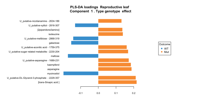
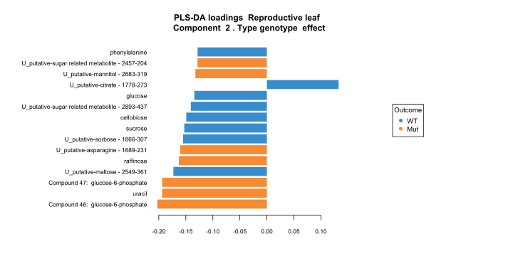
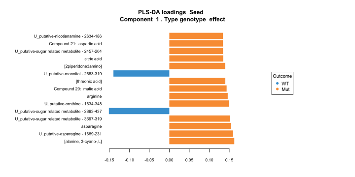
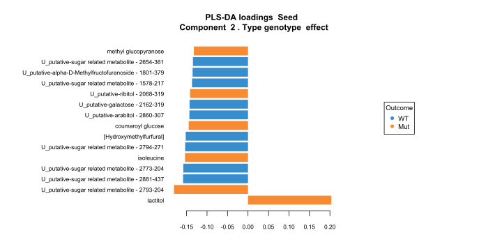
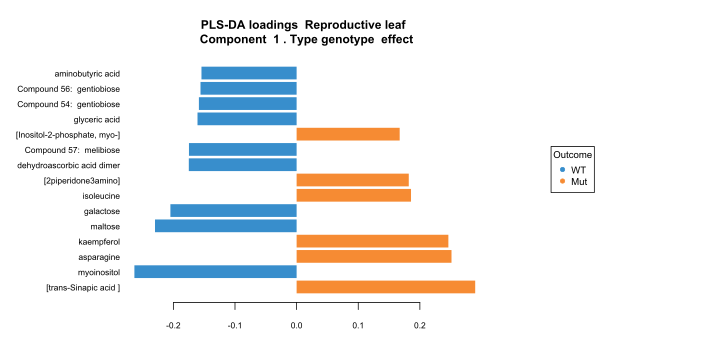
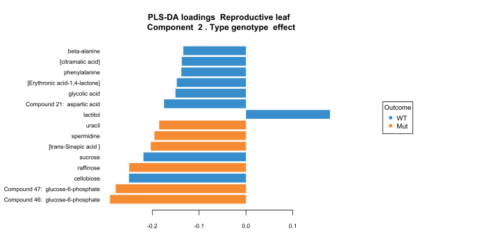
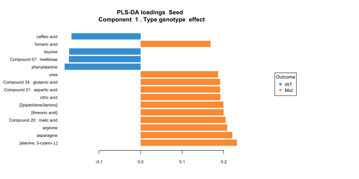
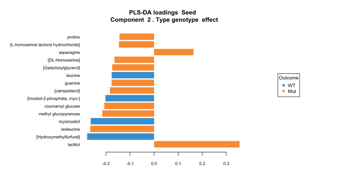
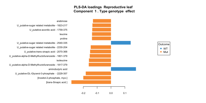
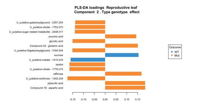
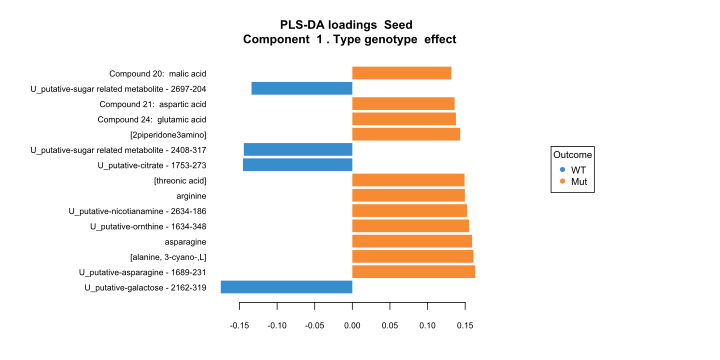
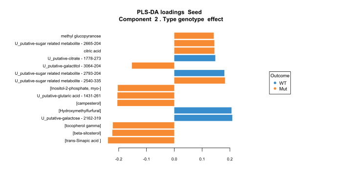
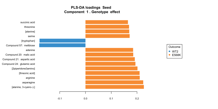
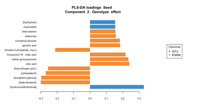
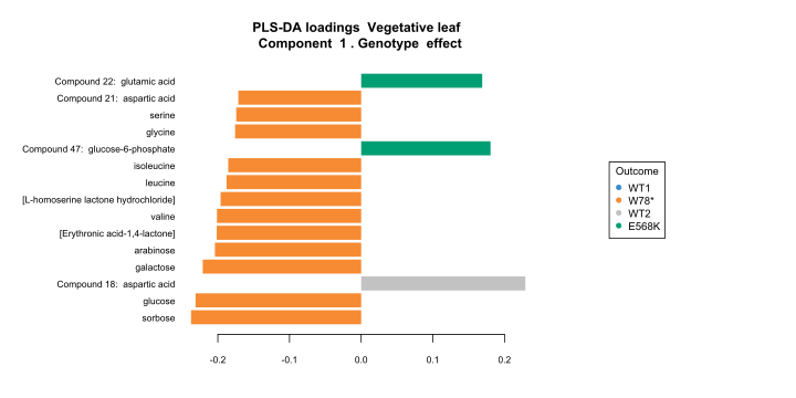
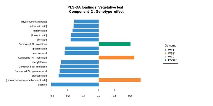
 Effect of the type of genotype