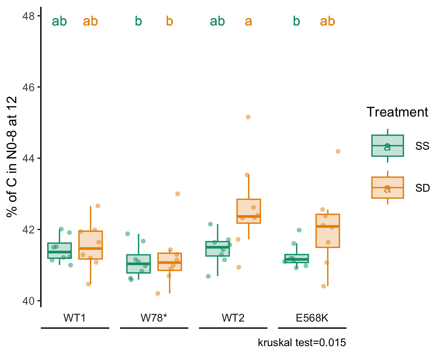
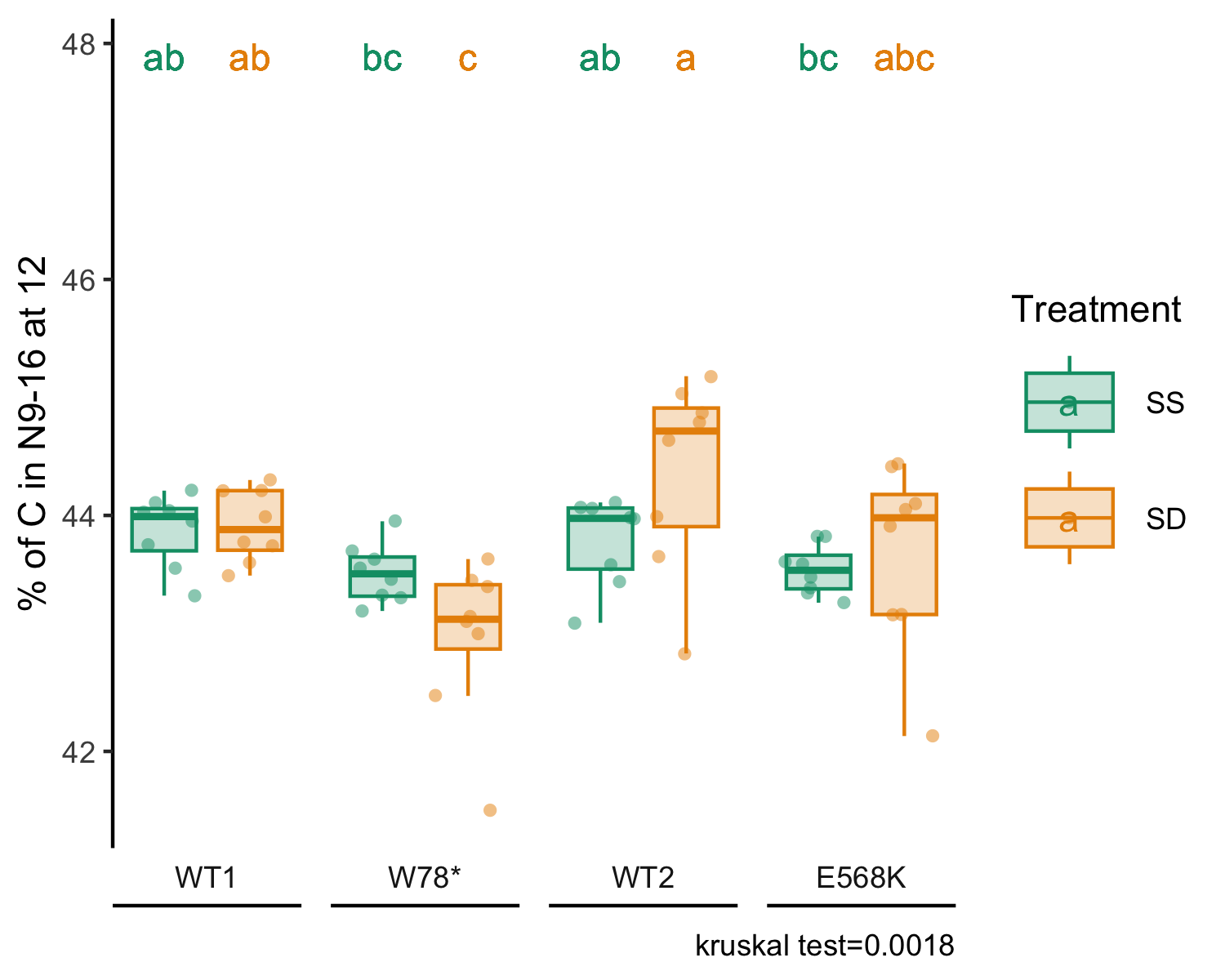
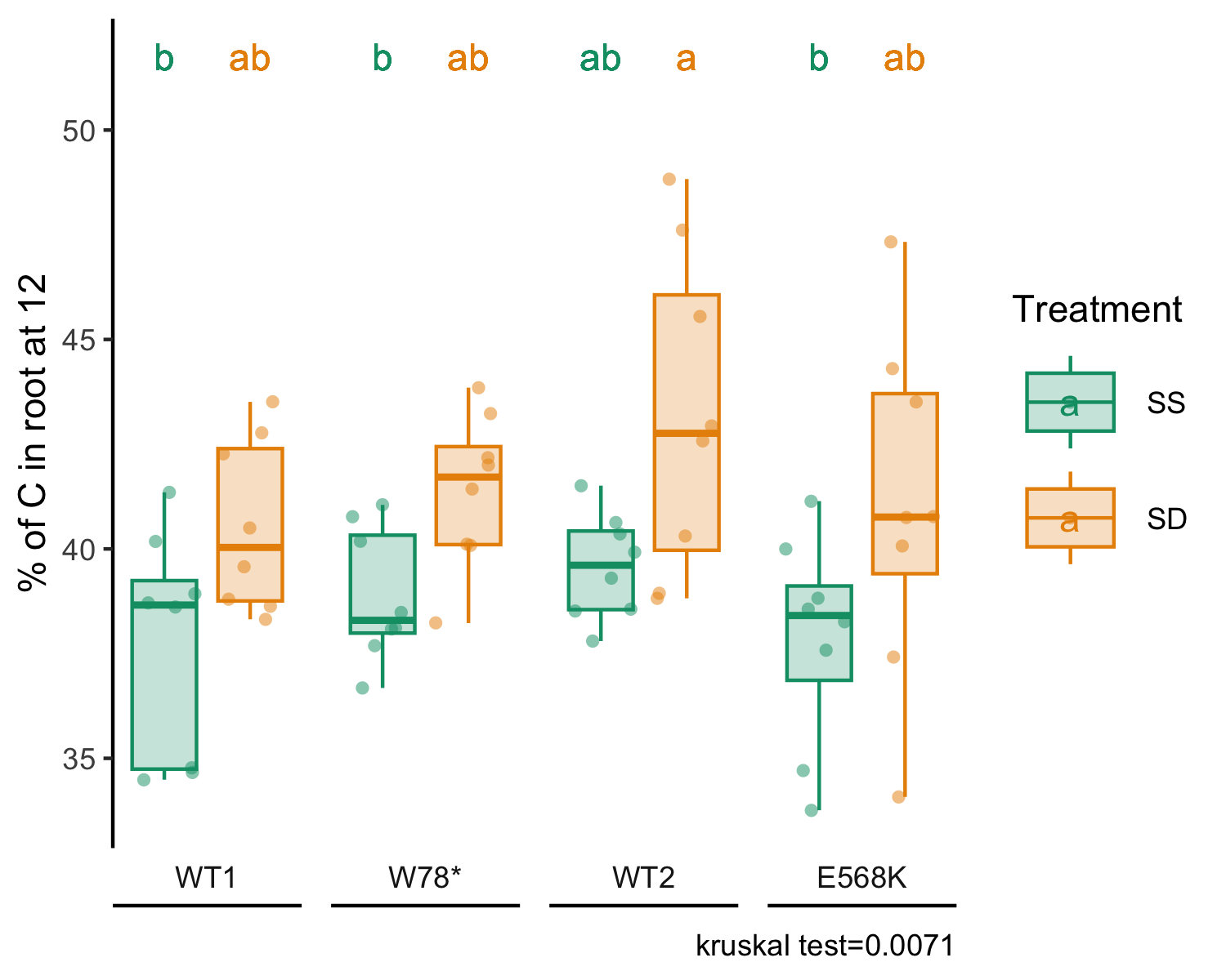
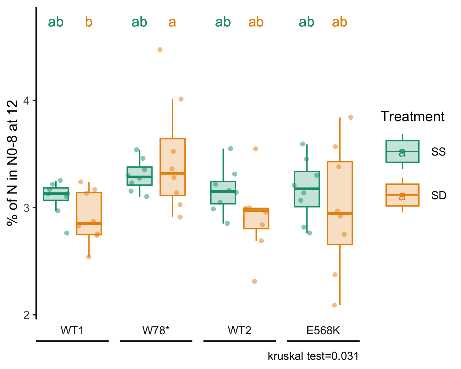
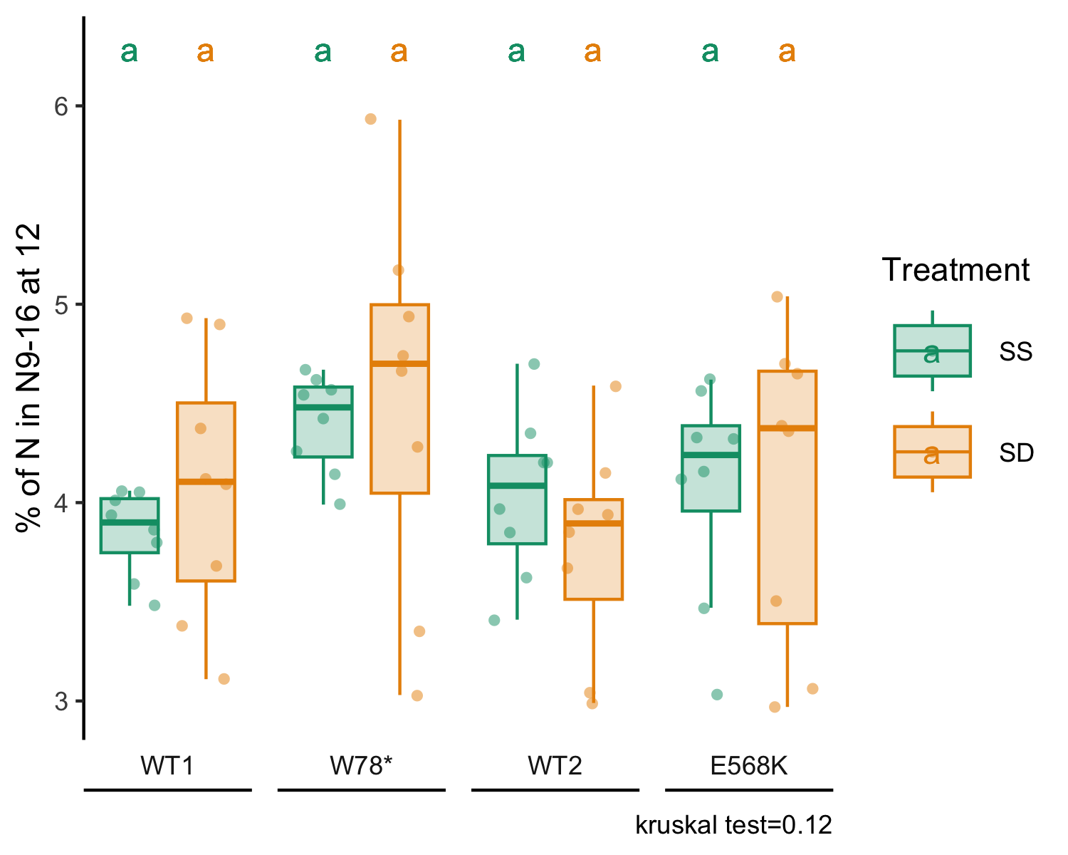
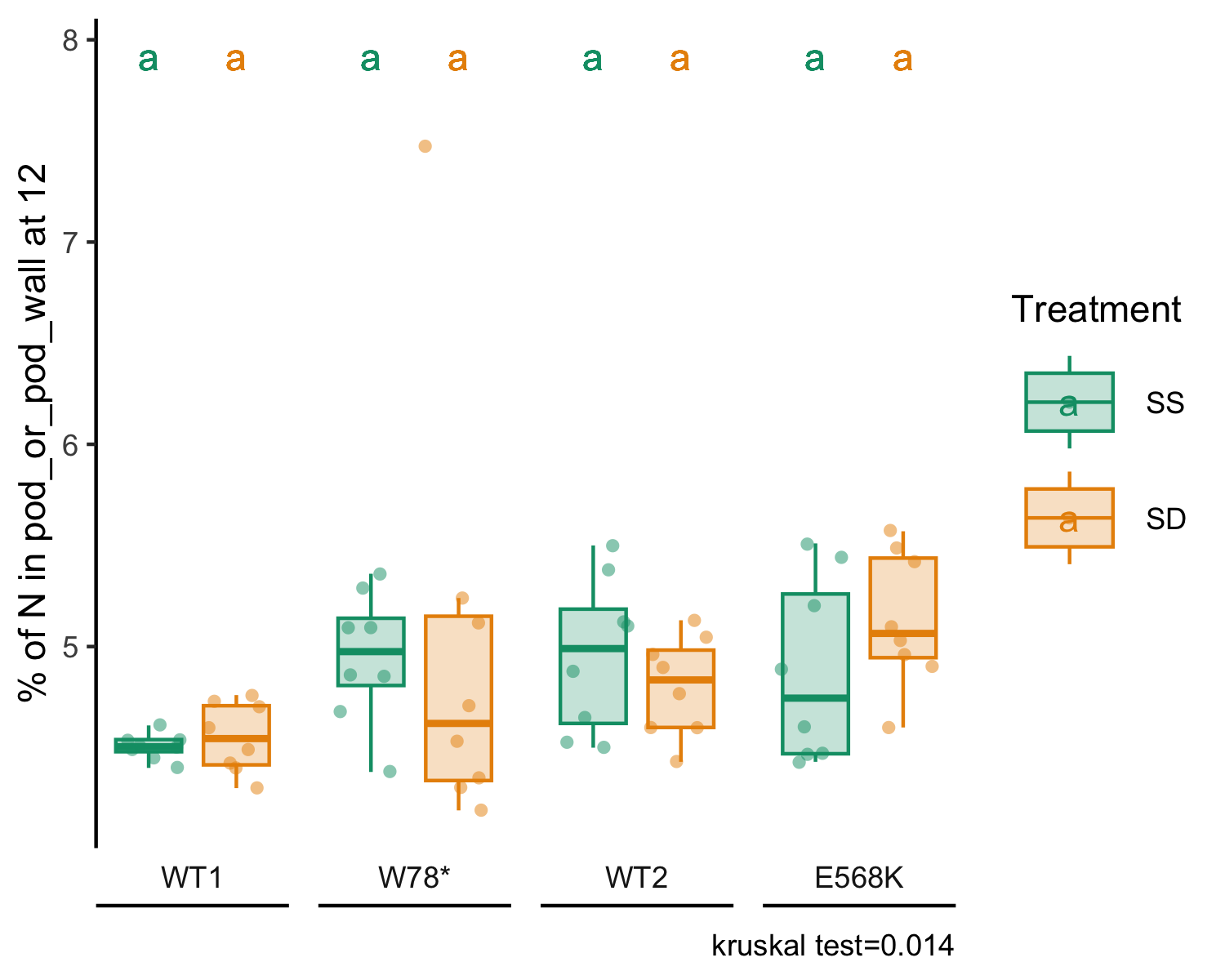
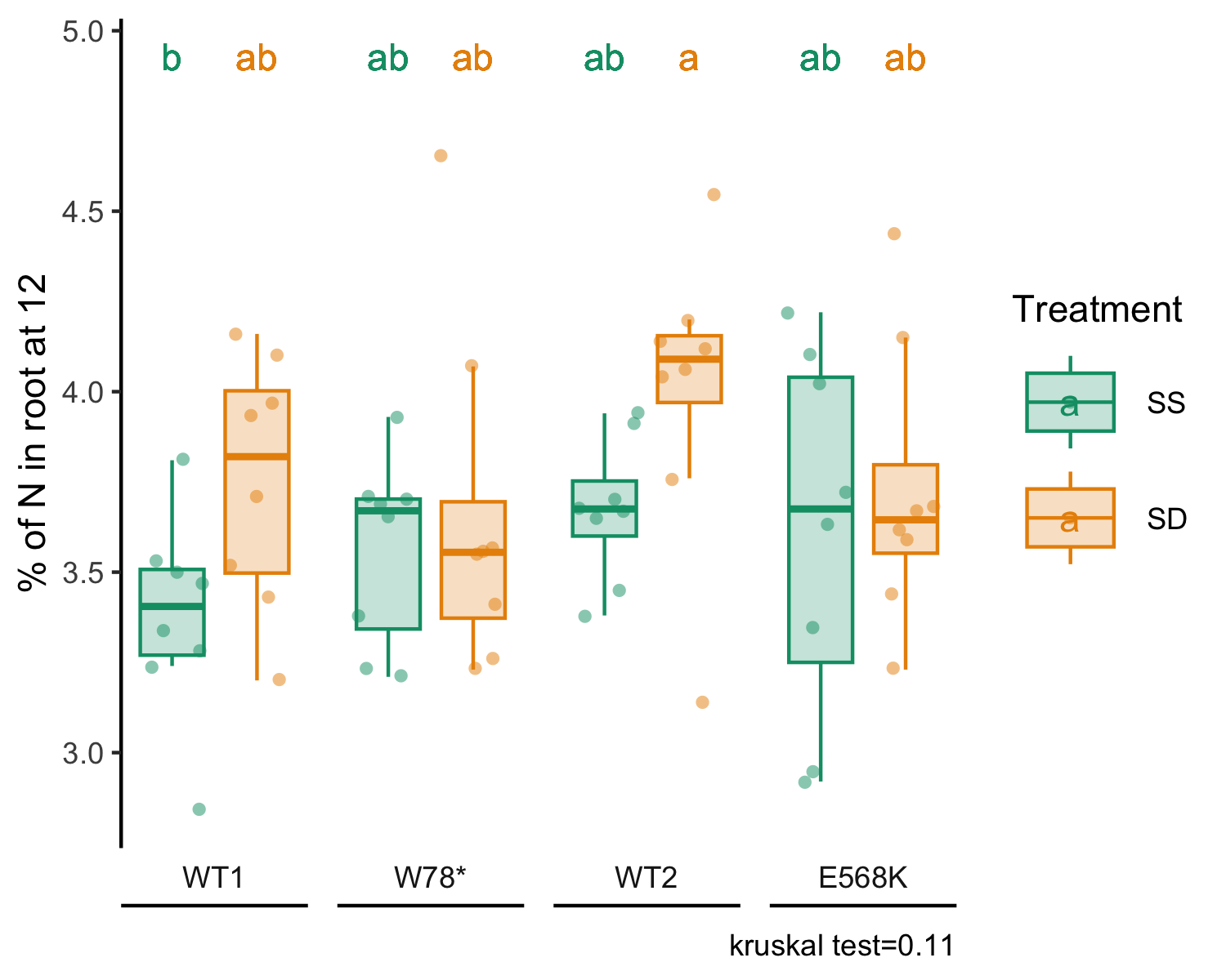
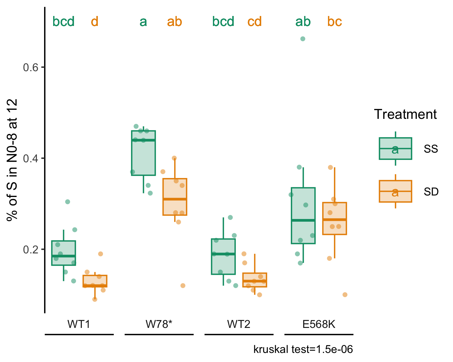
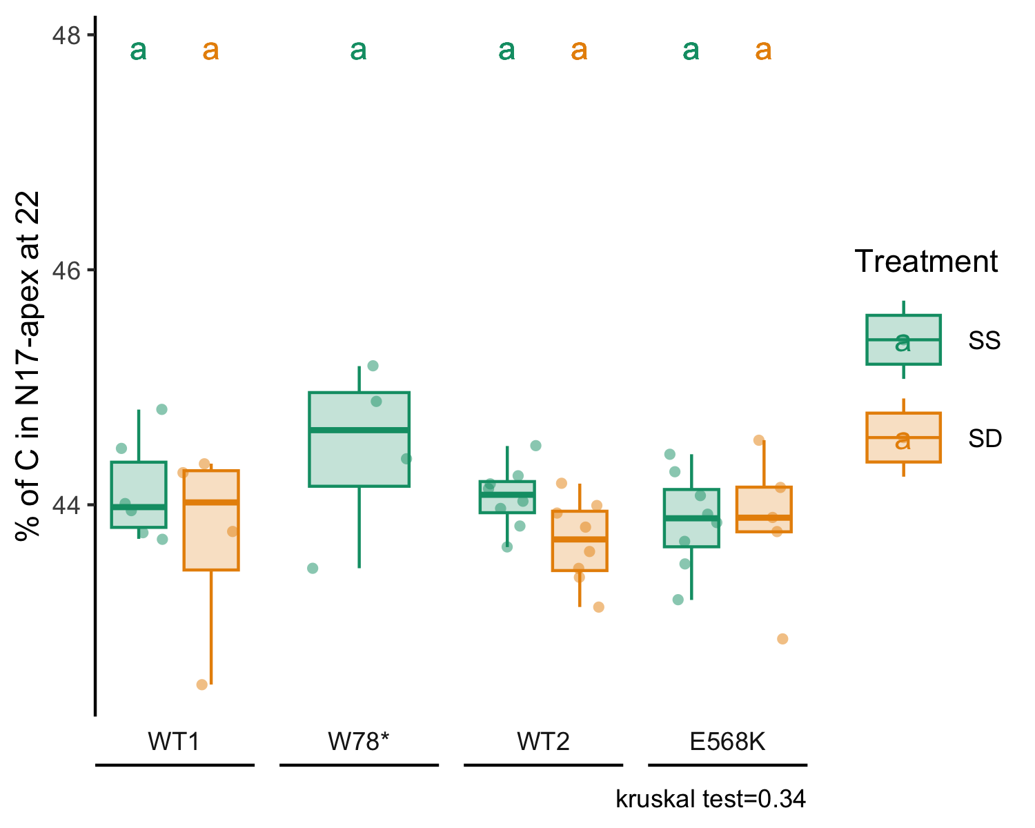
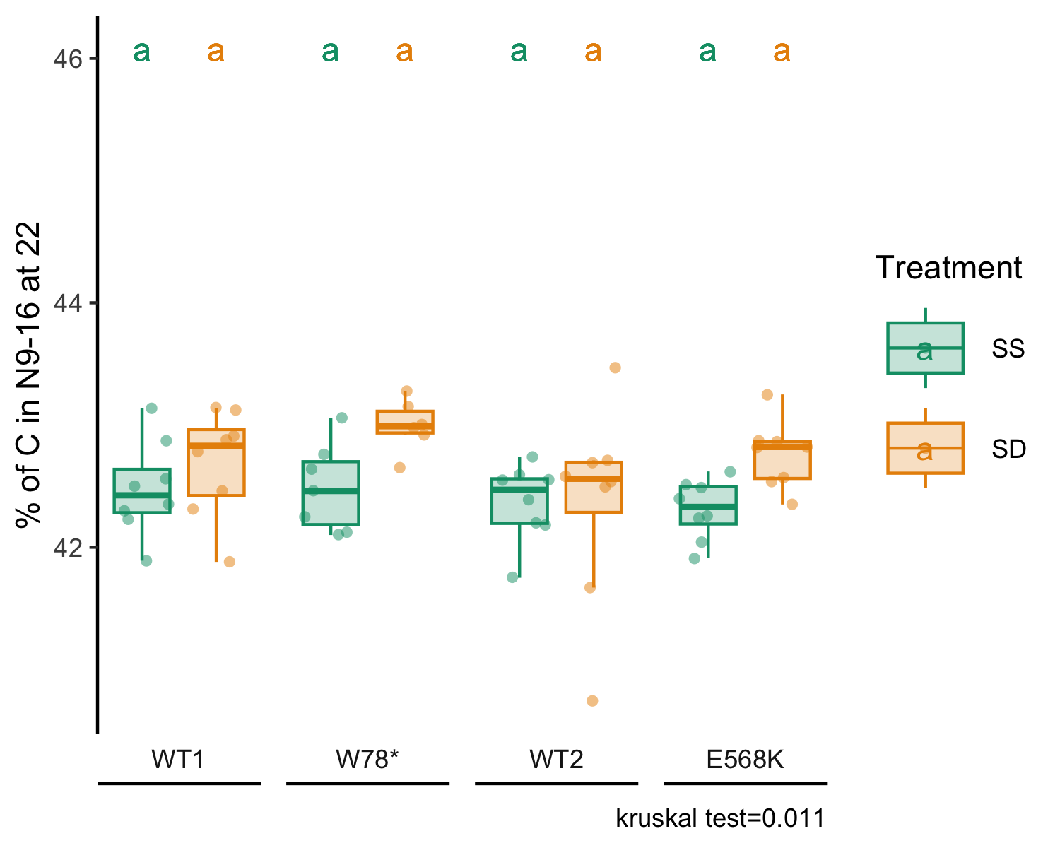
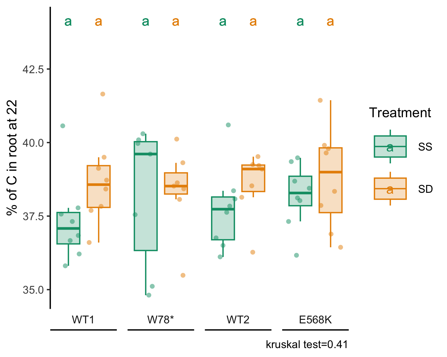
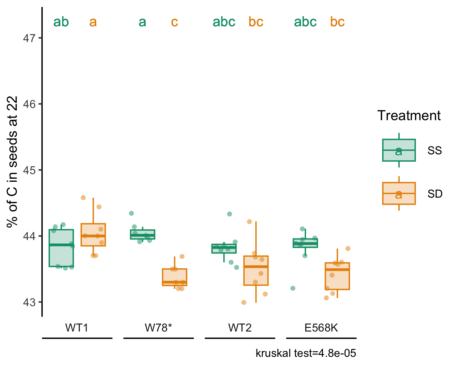
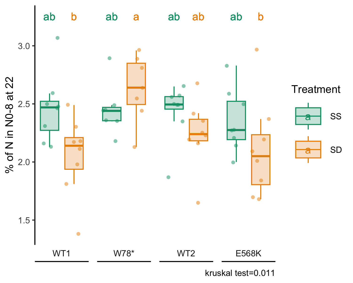
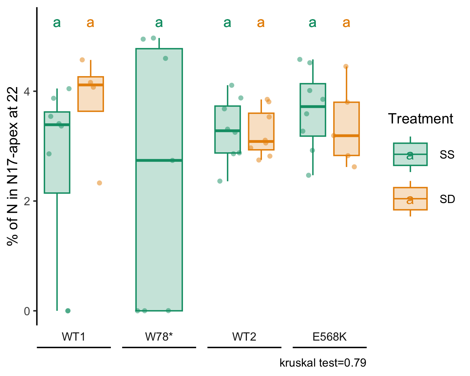
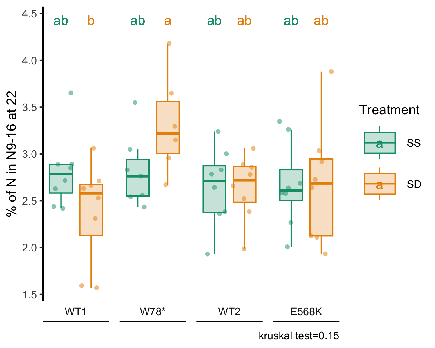
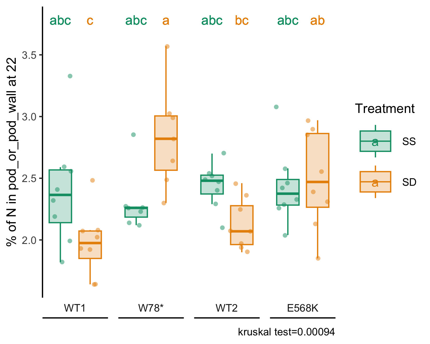
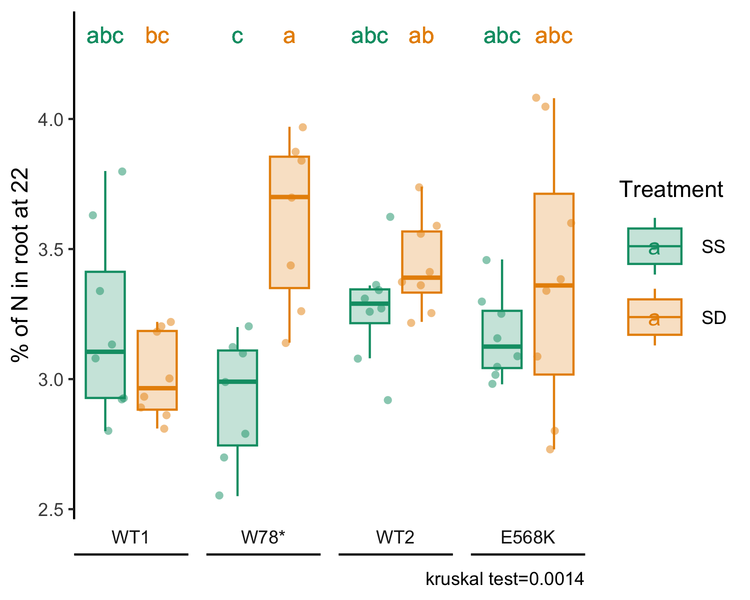
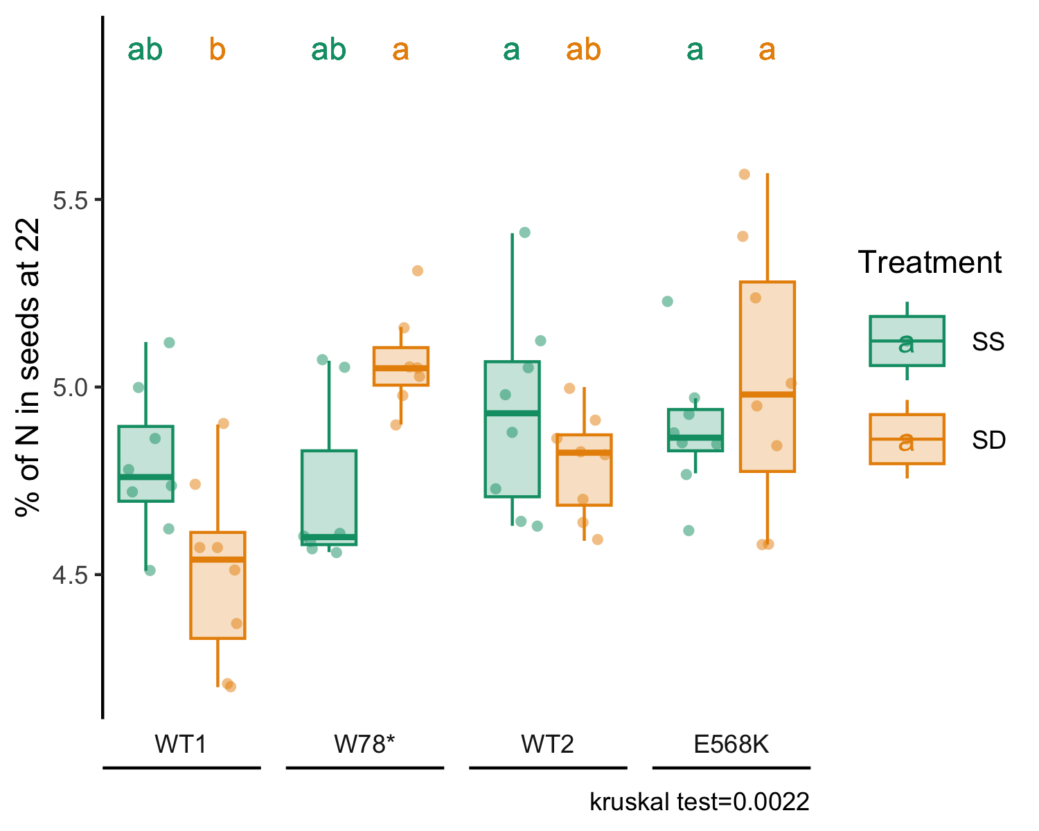
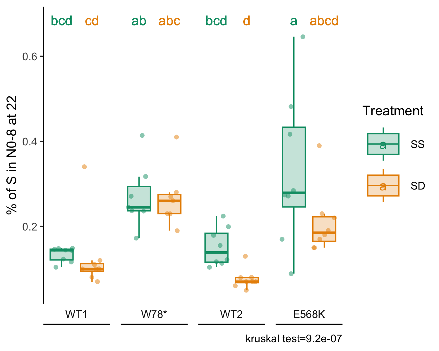
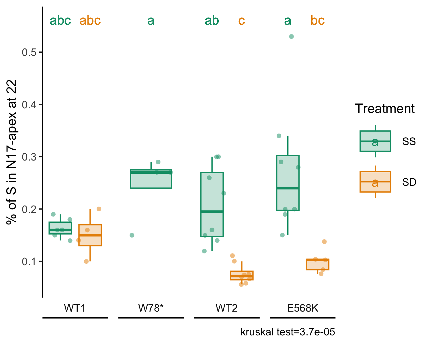
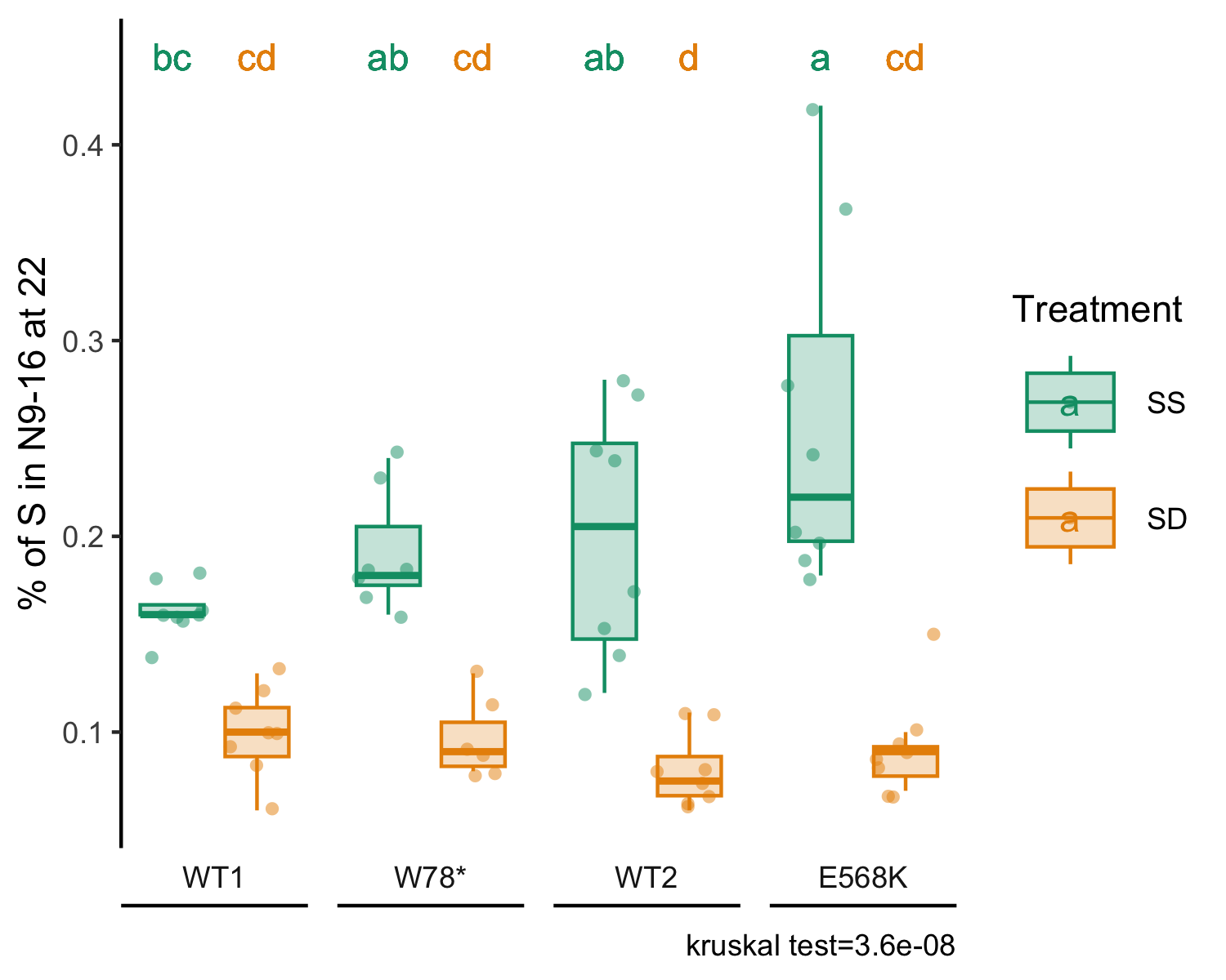
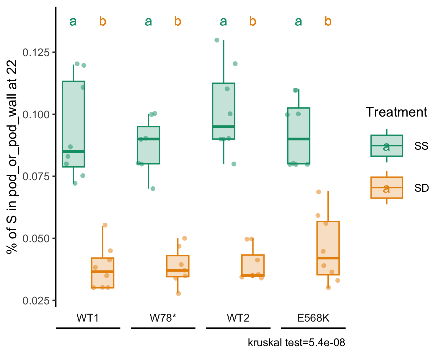
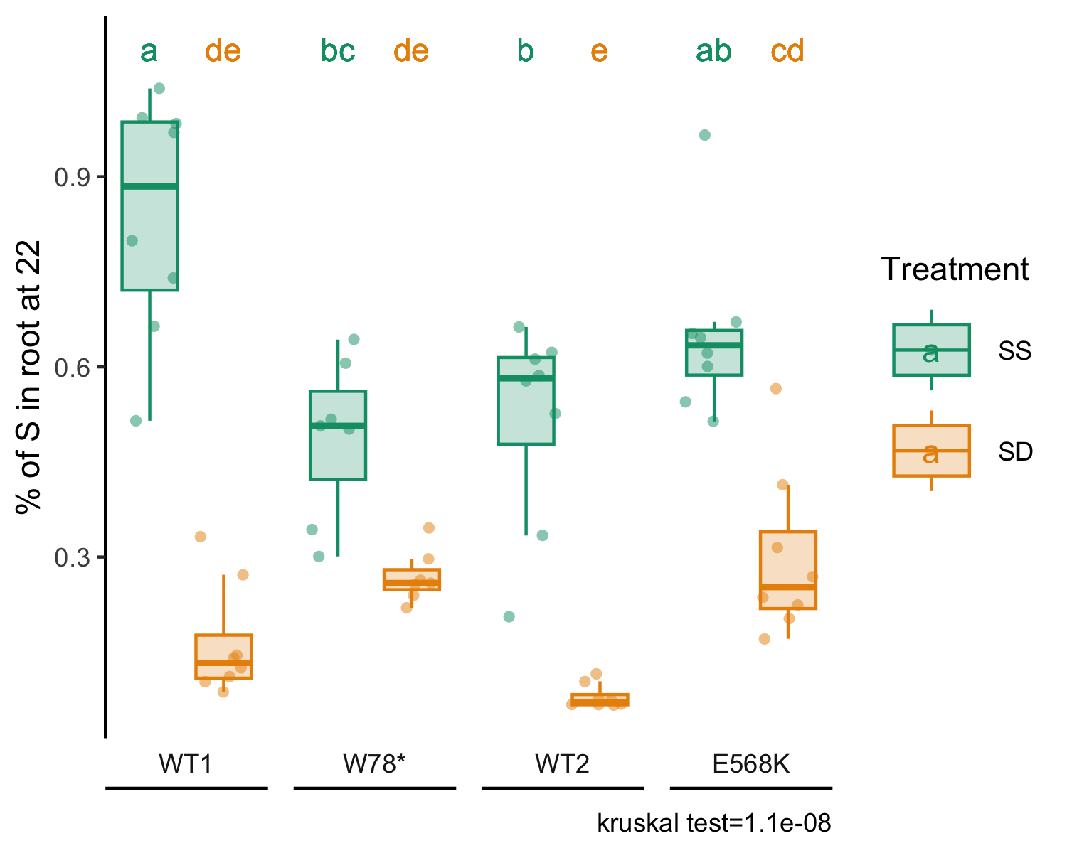
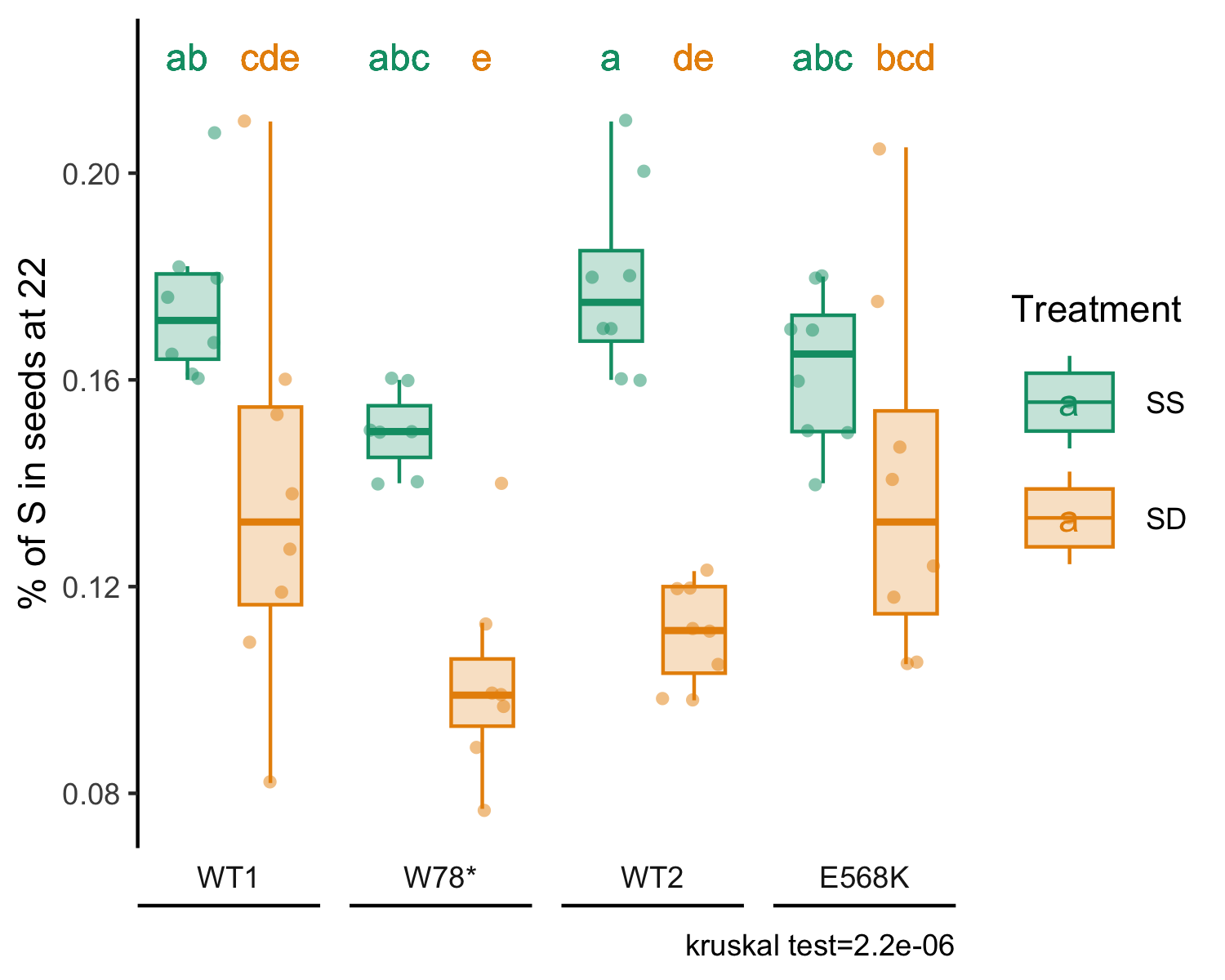
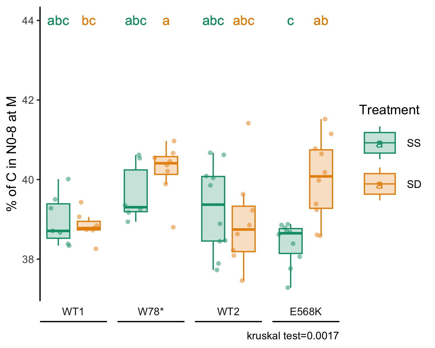
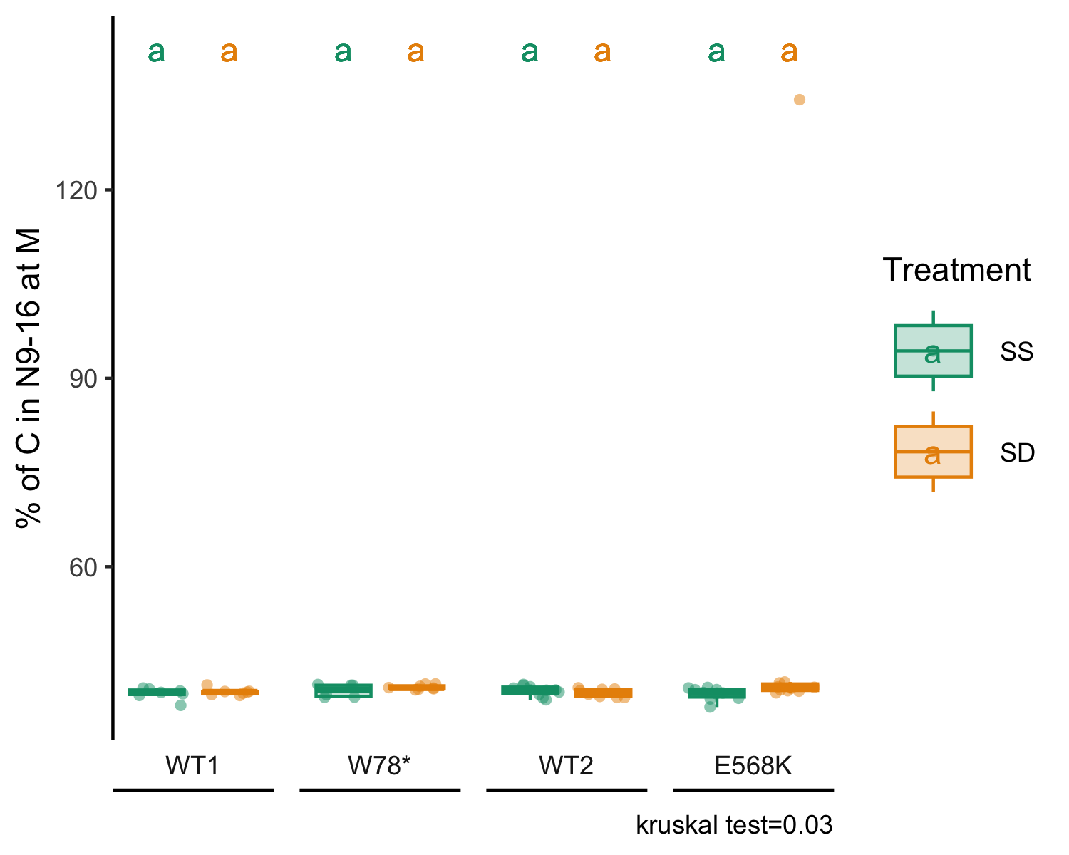
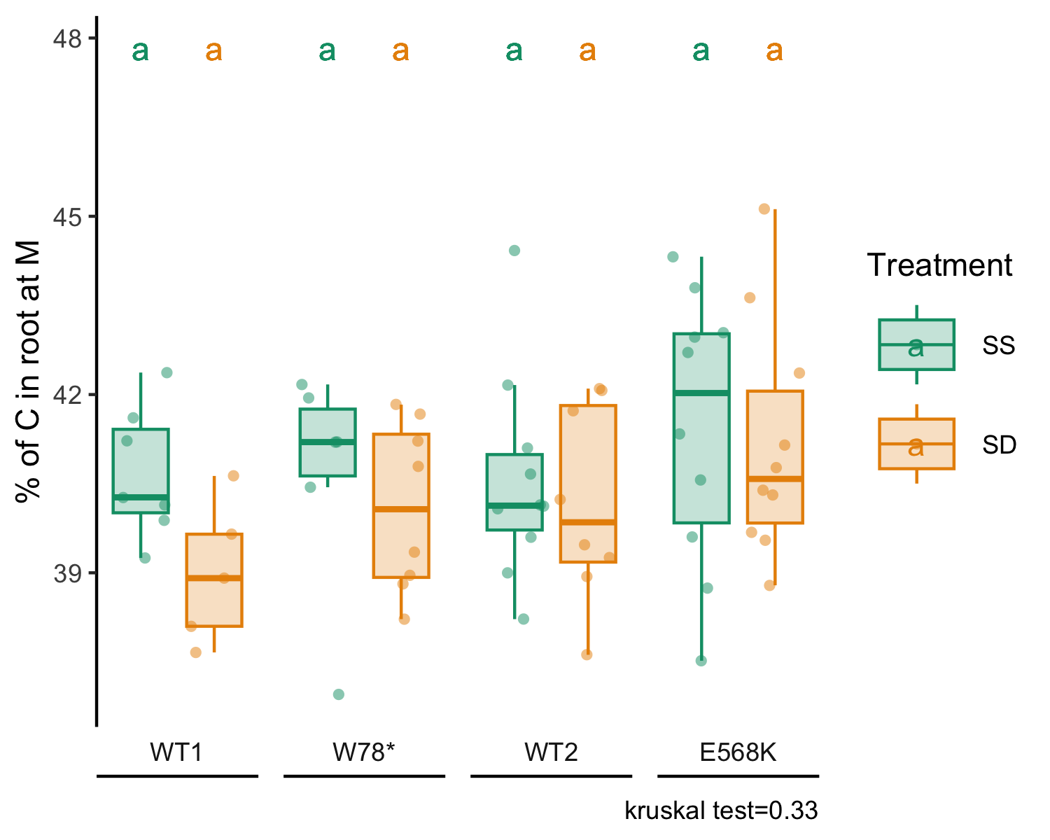
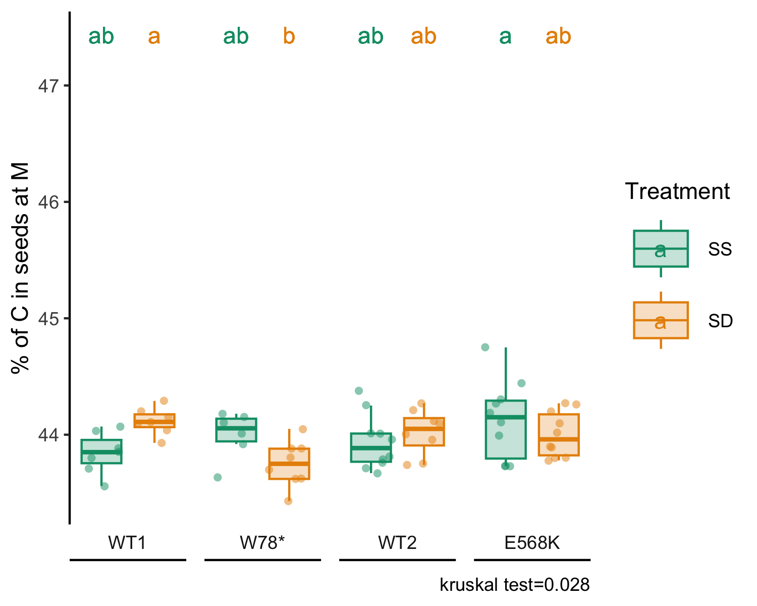
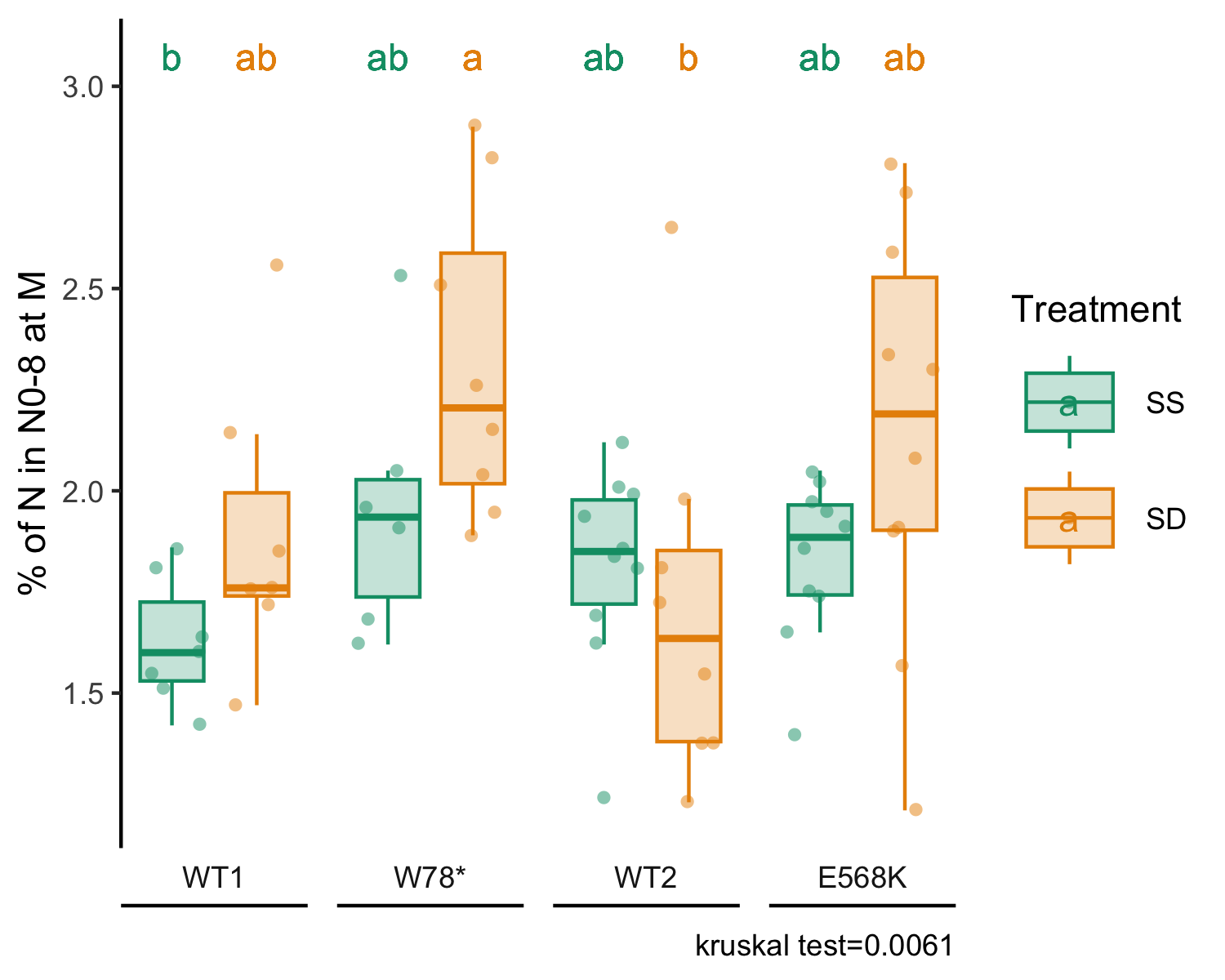
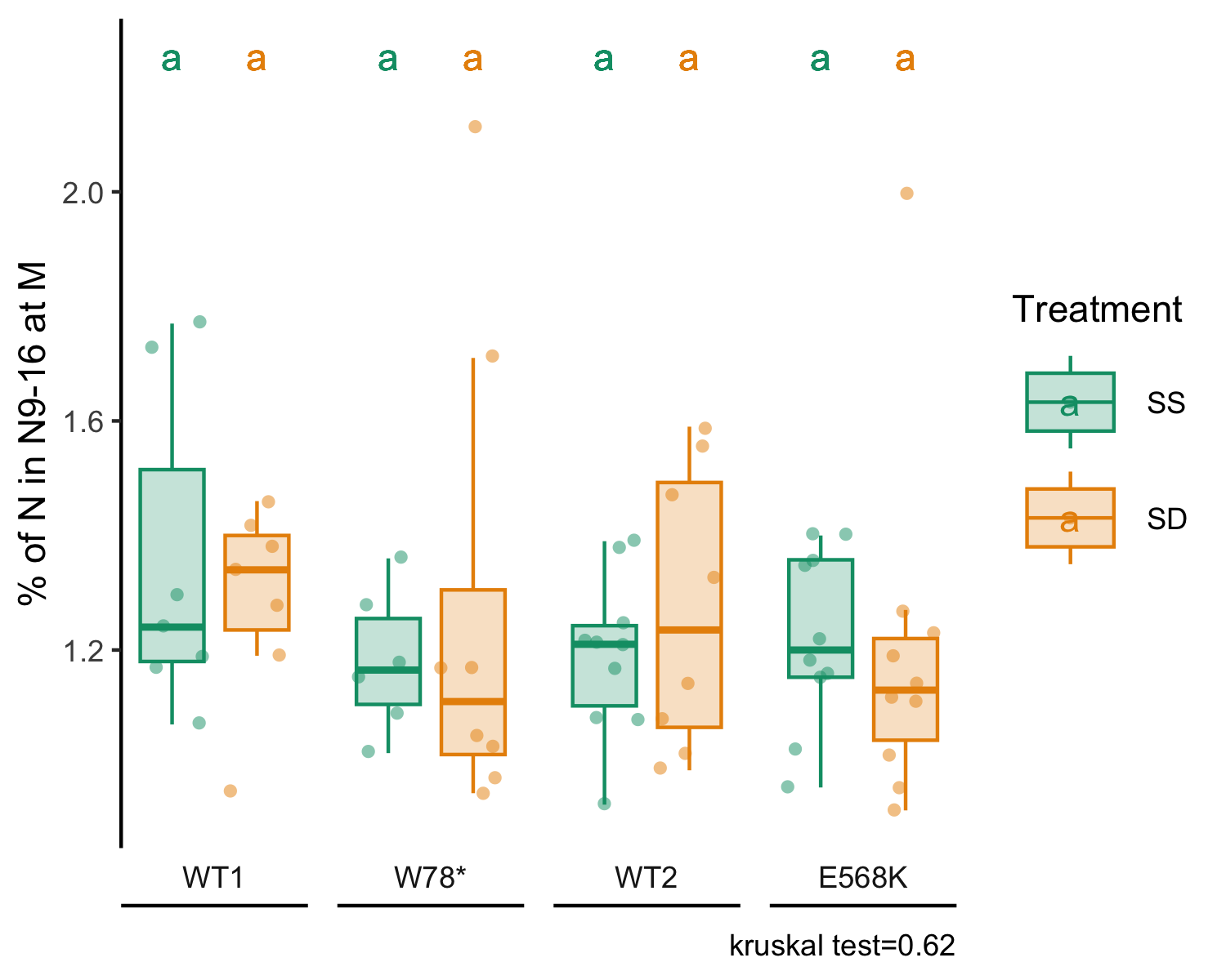
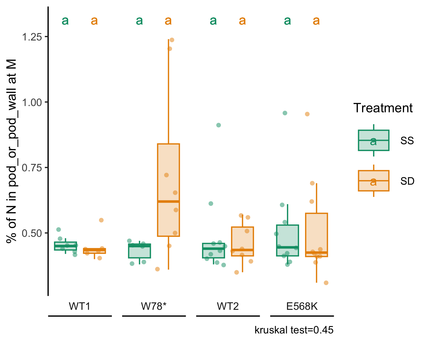
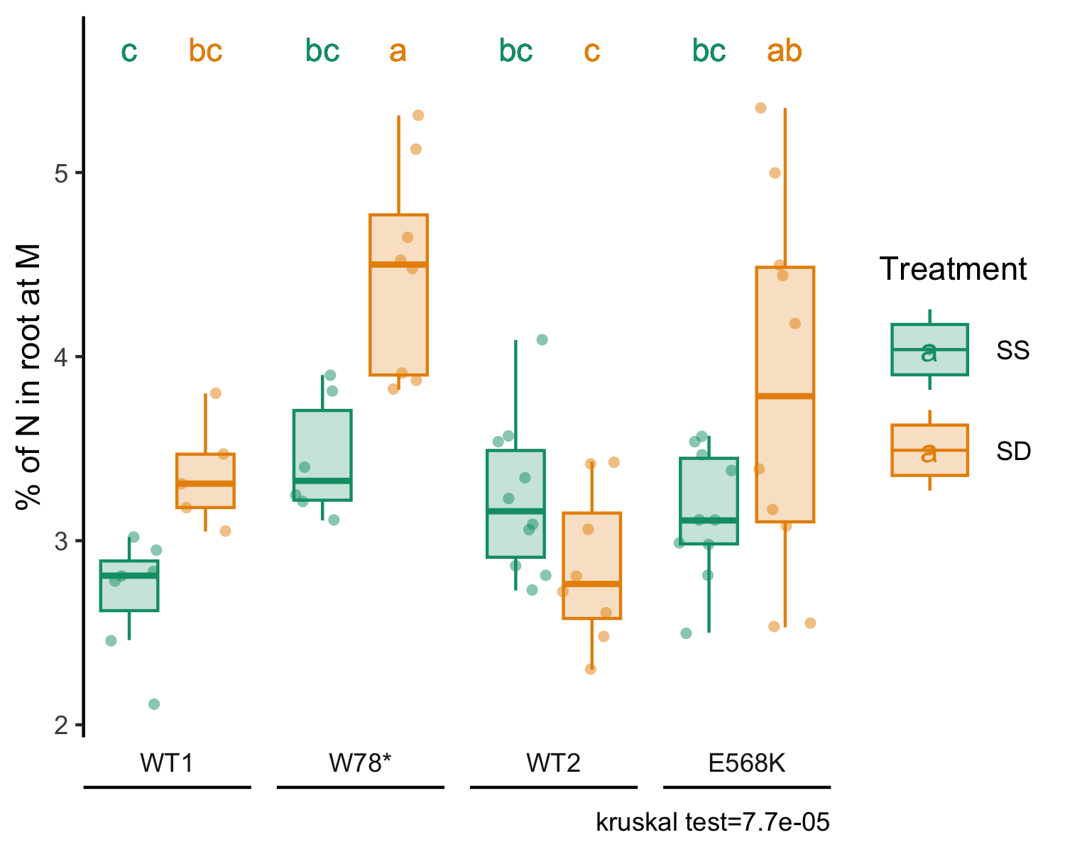
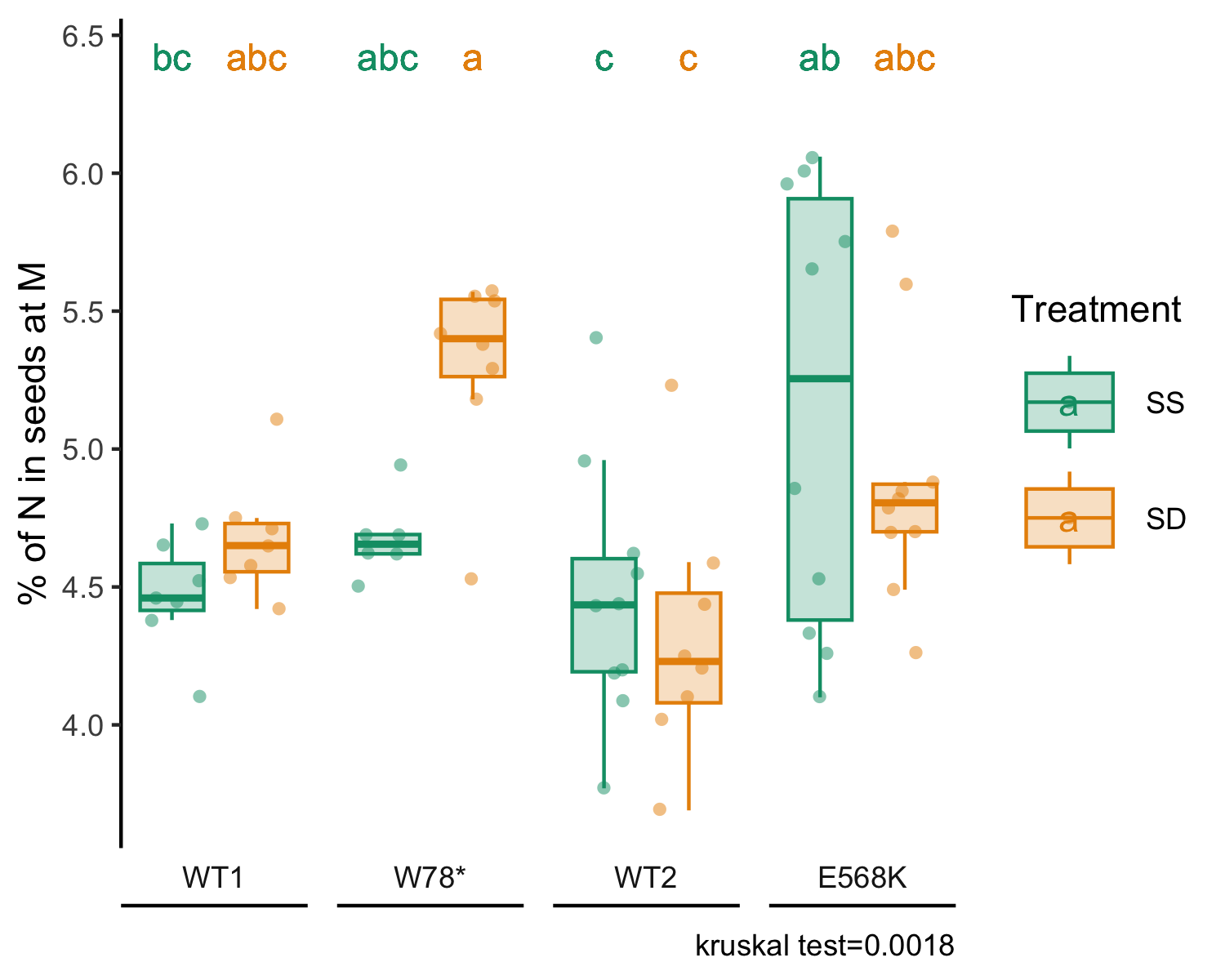
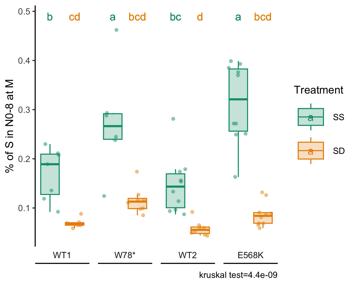
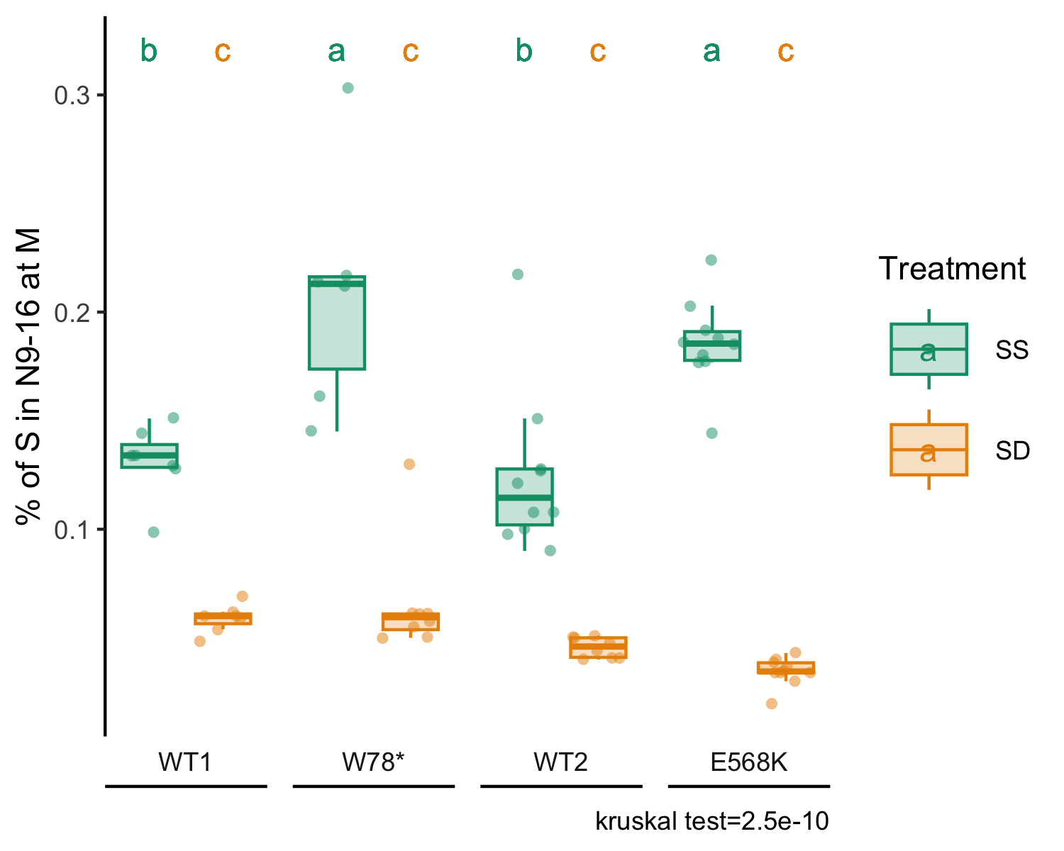
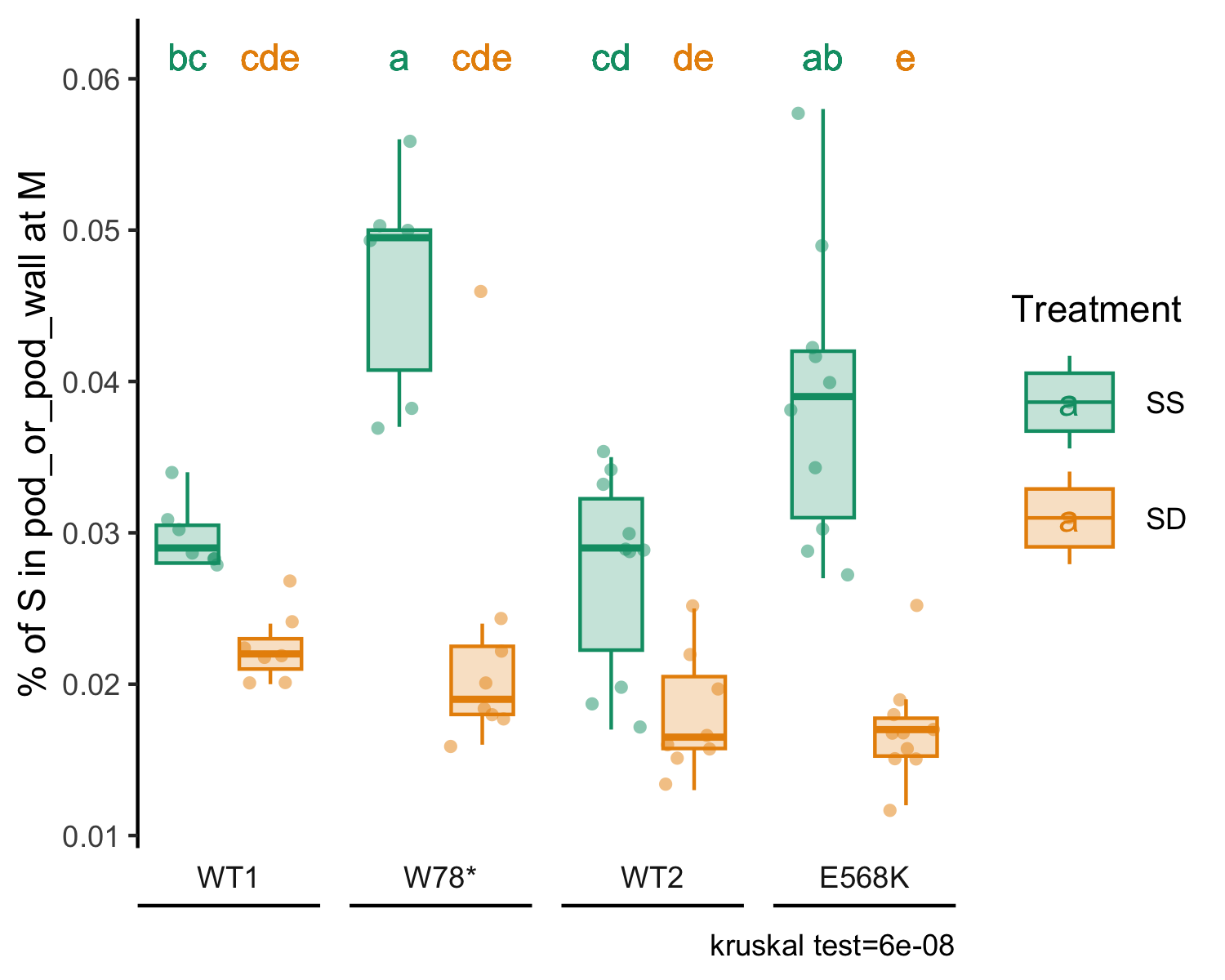
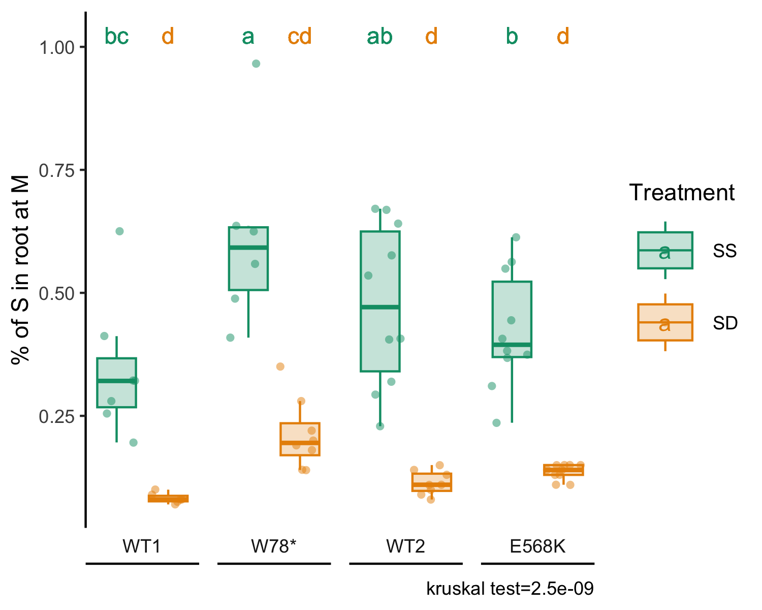
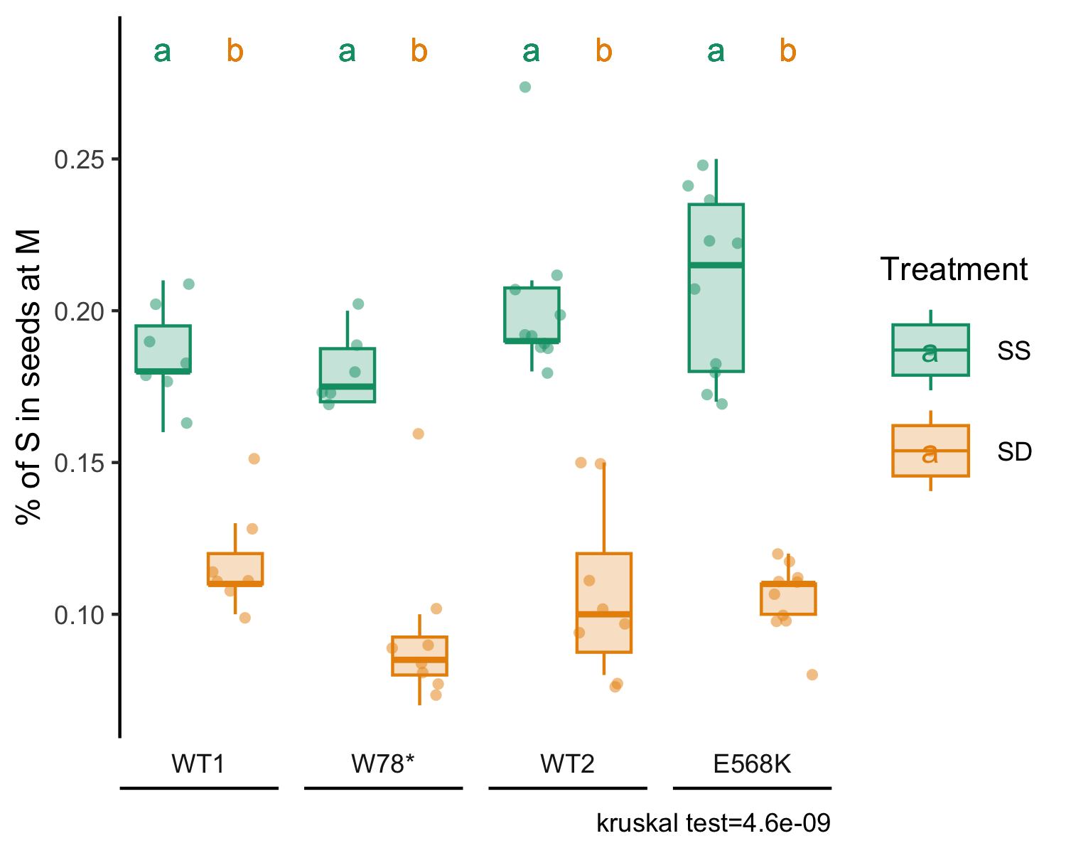
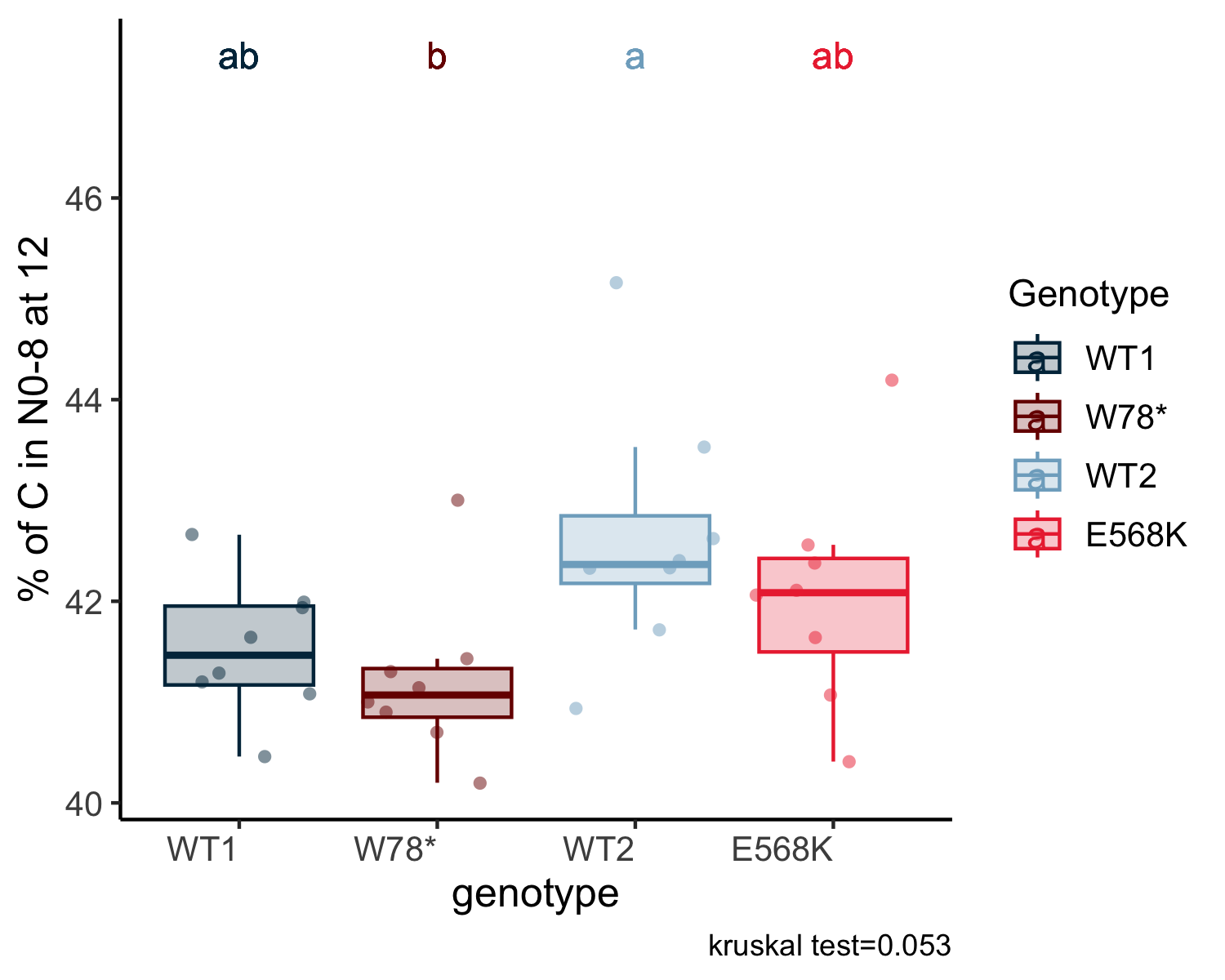
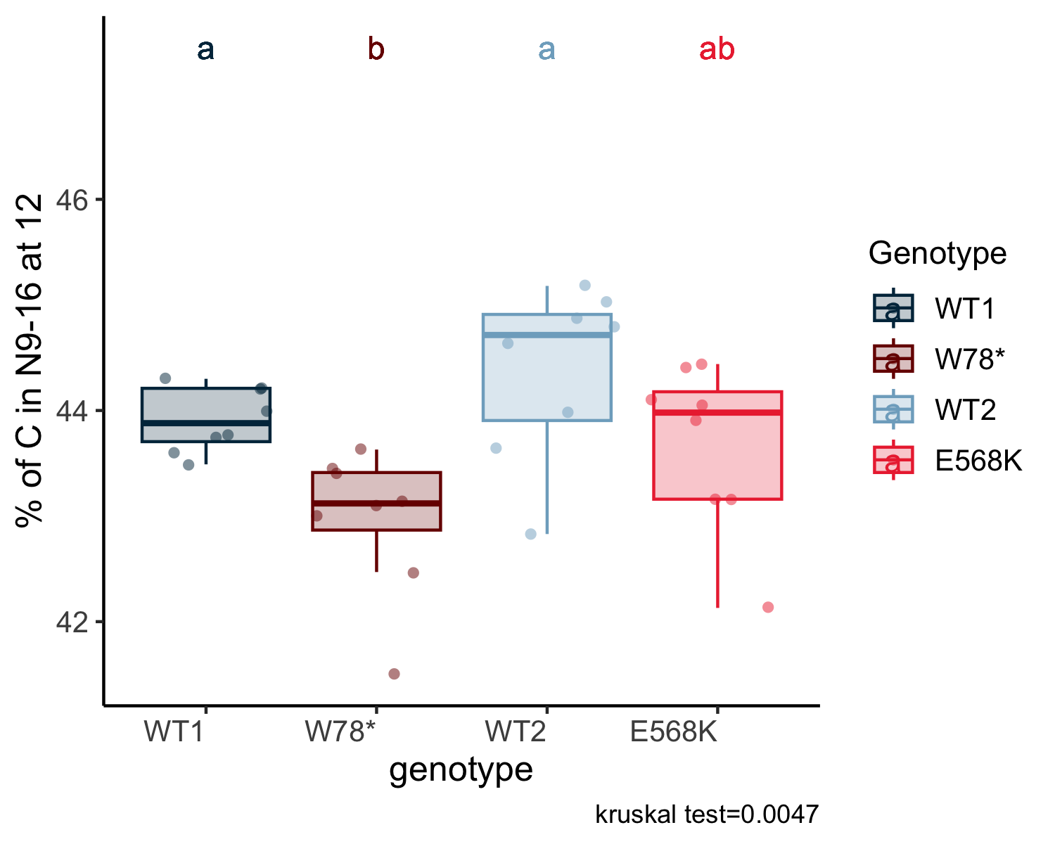
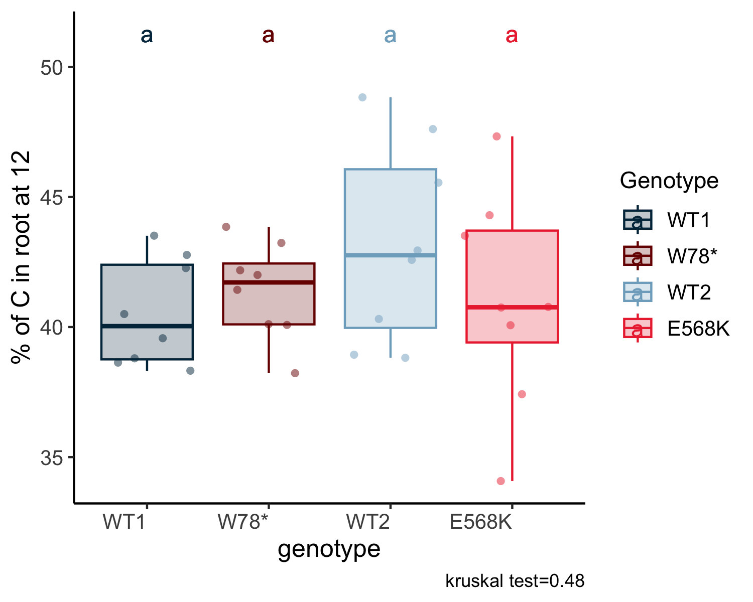
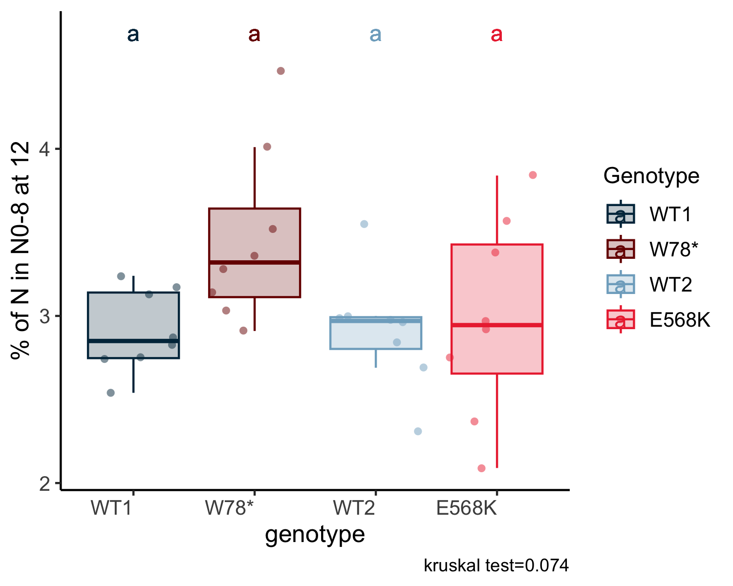
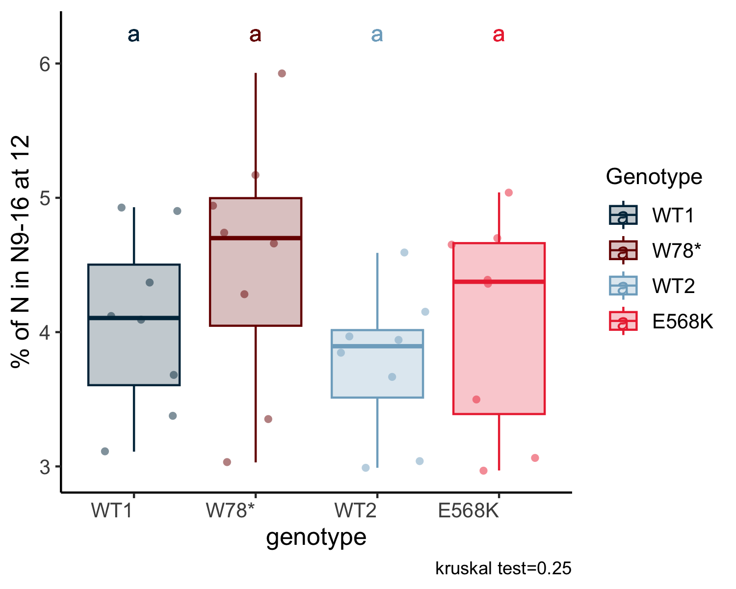
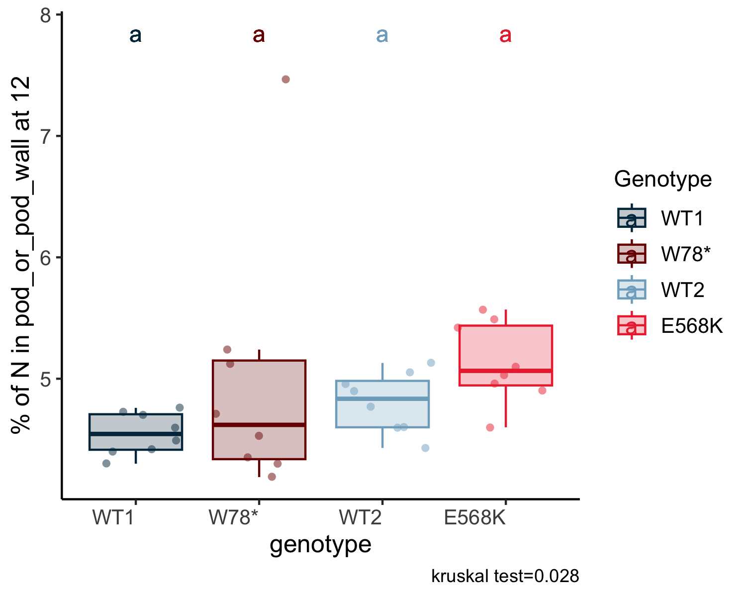
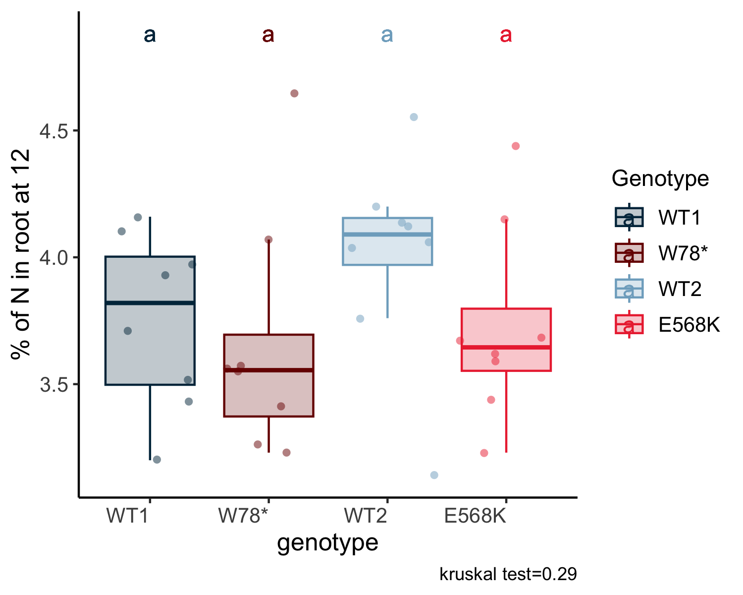
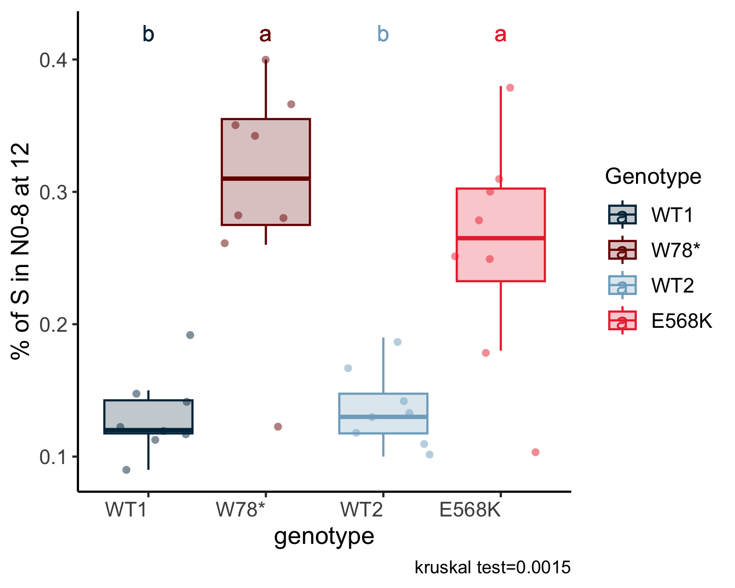
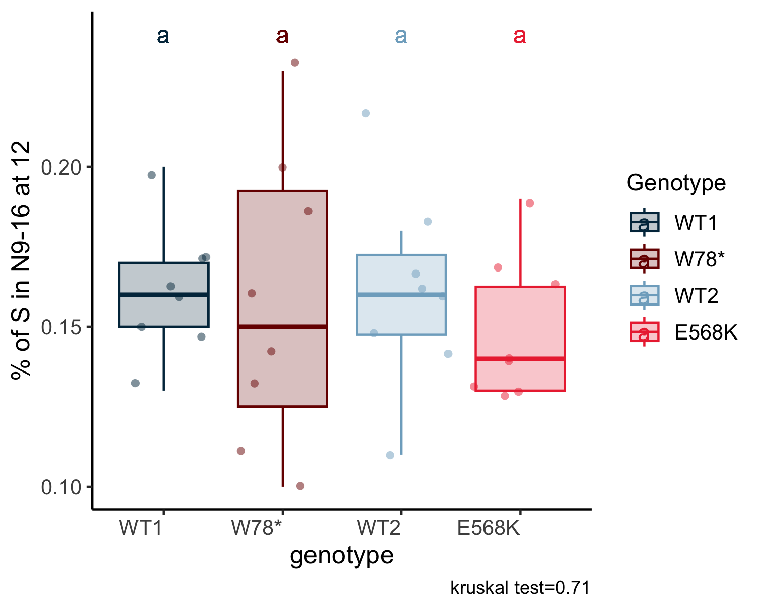
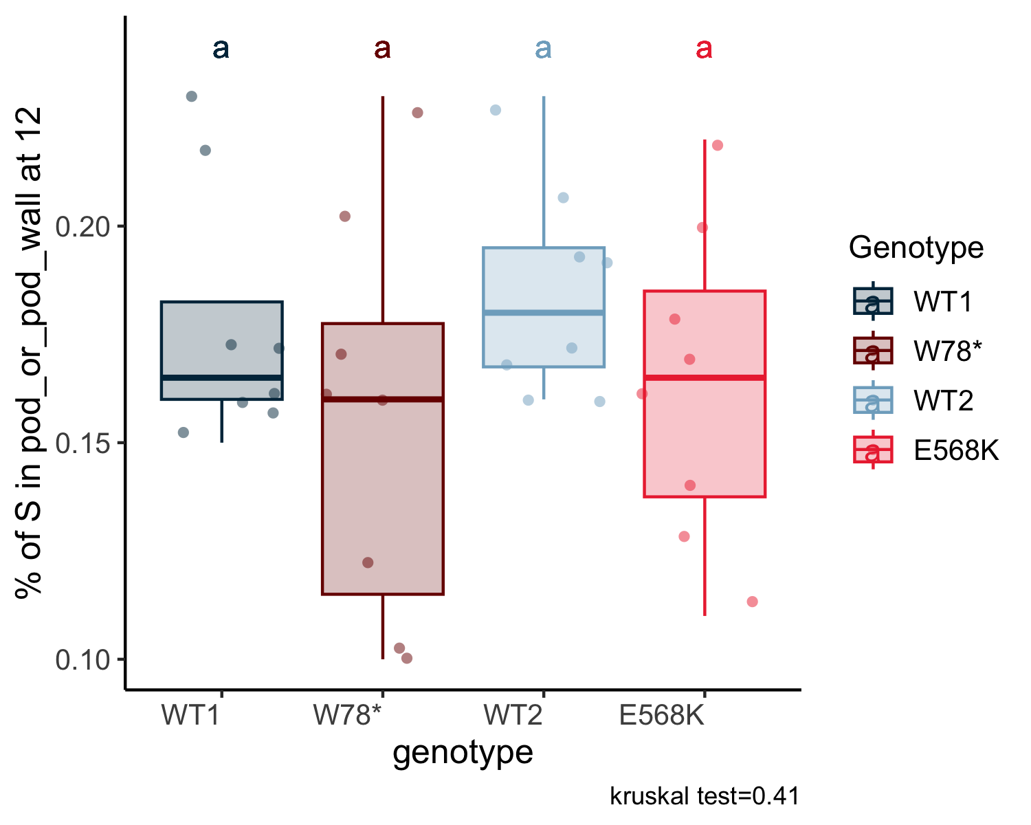
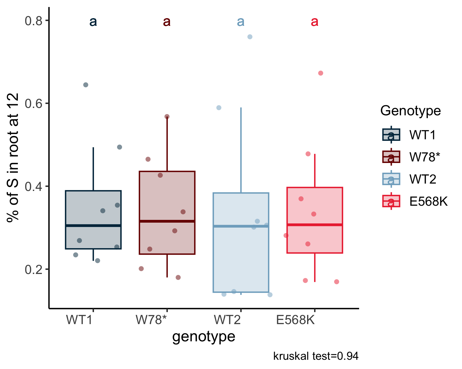
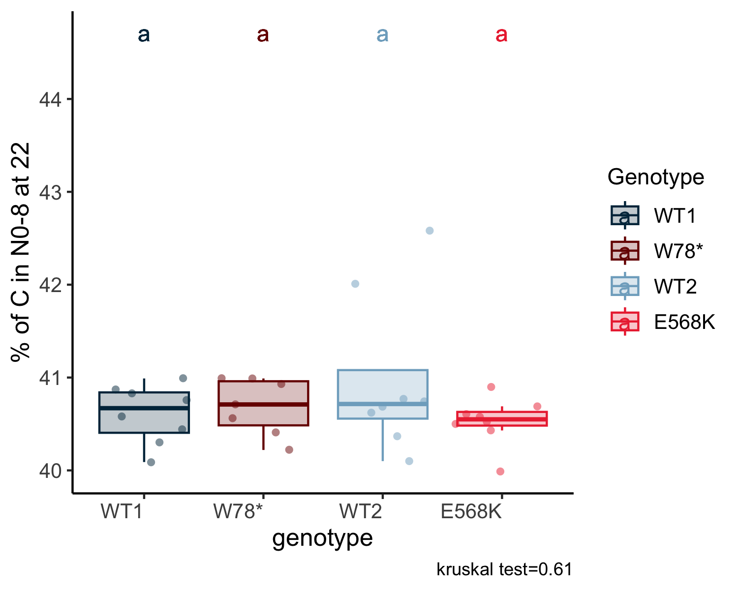
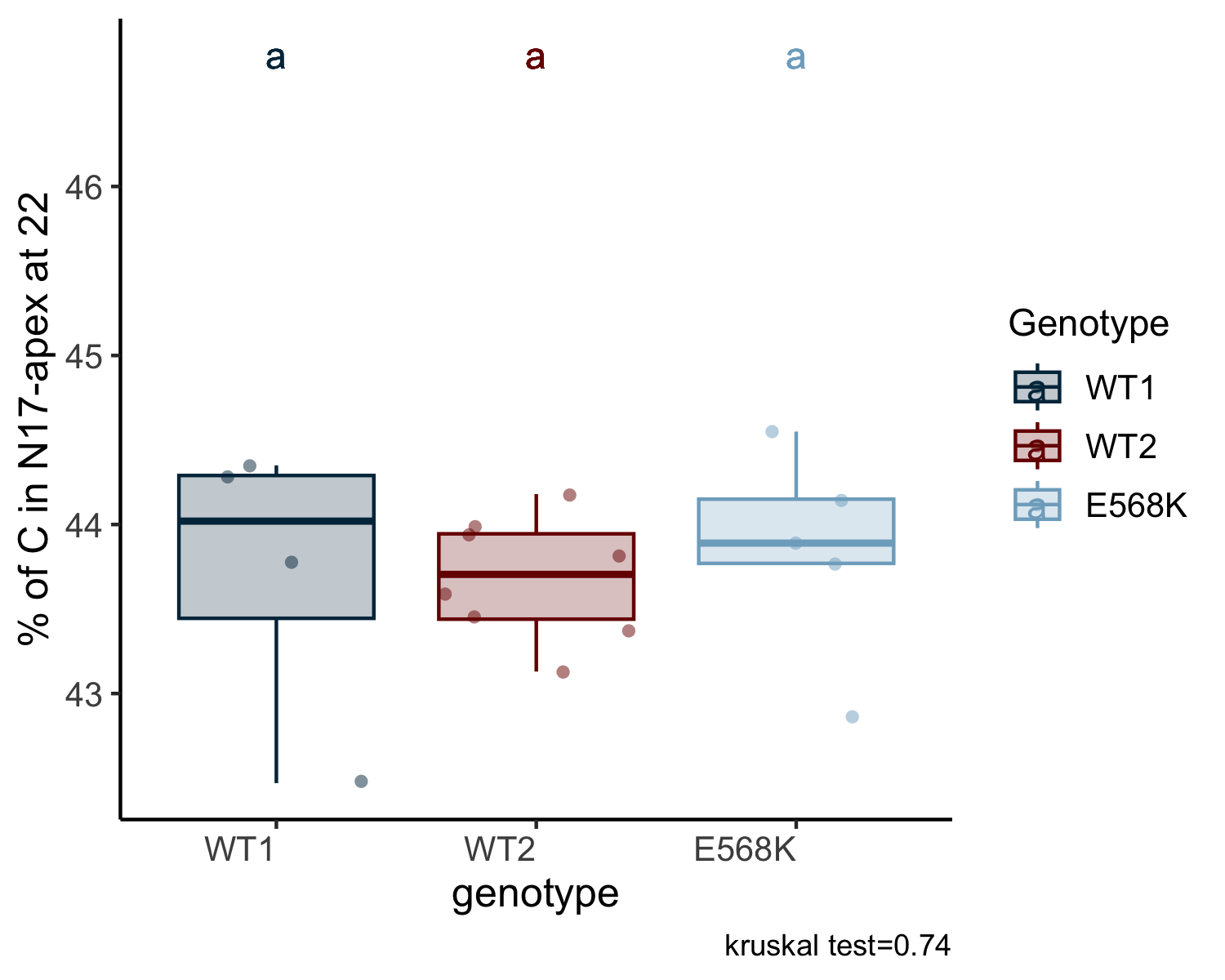
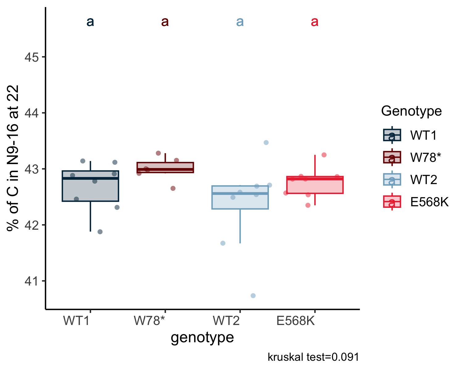
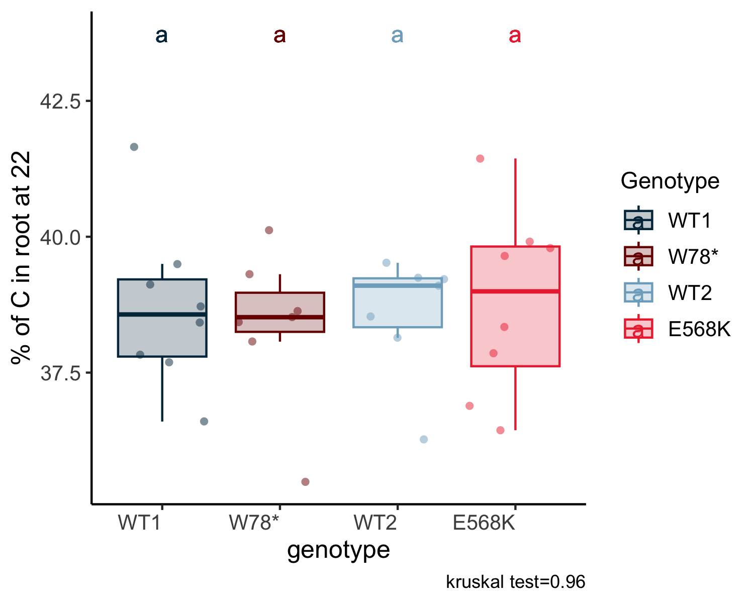
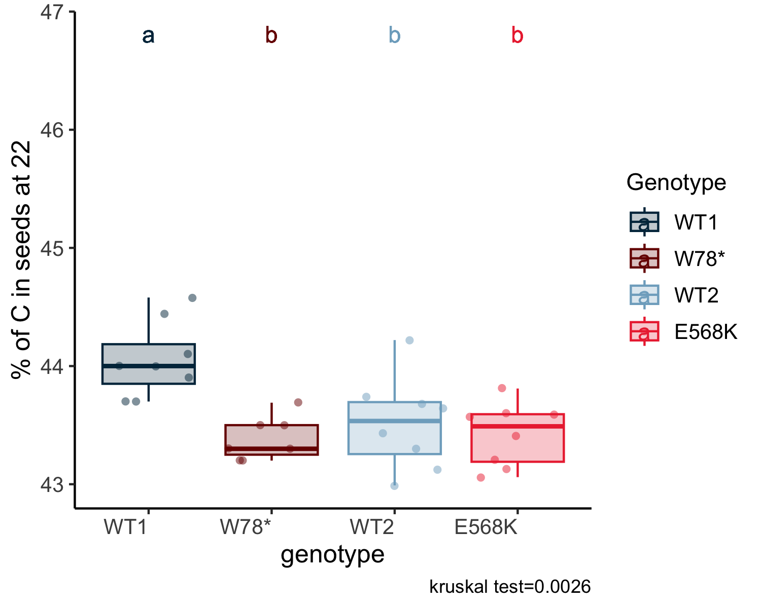
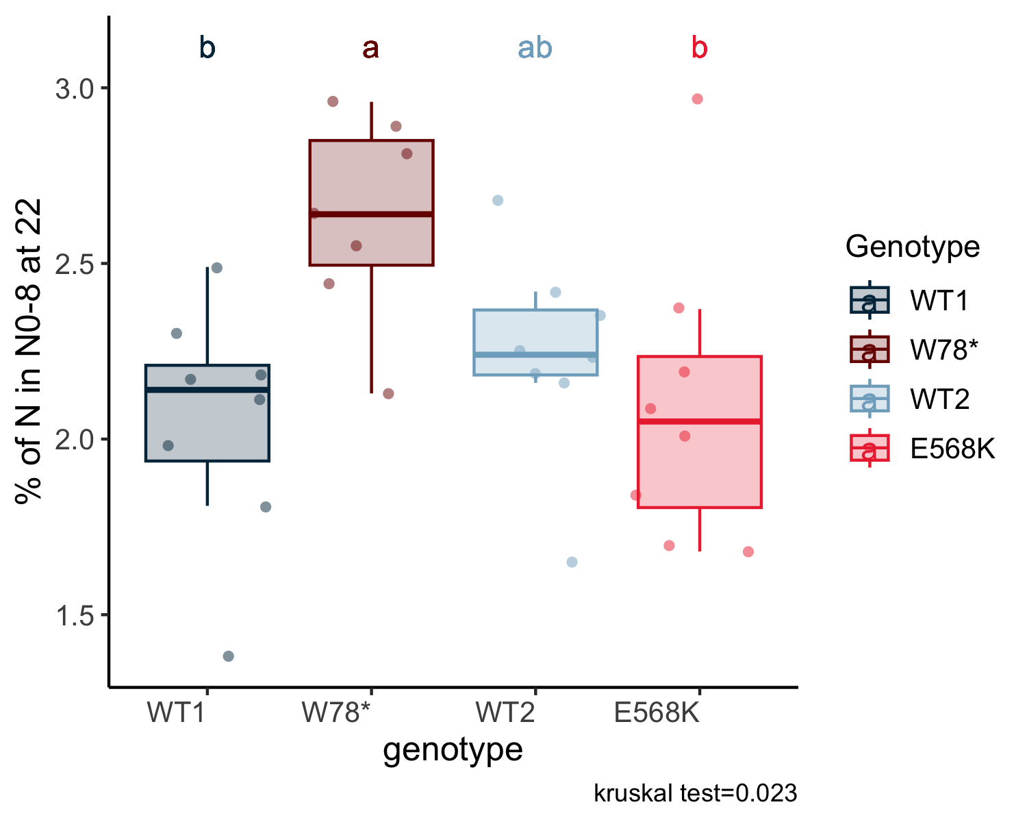
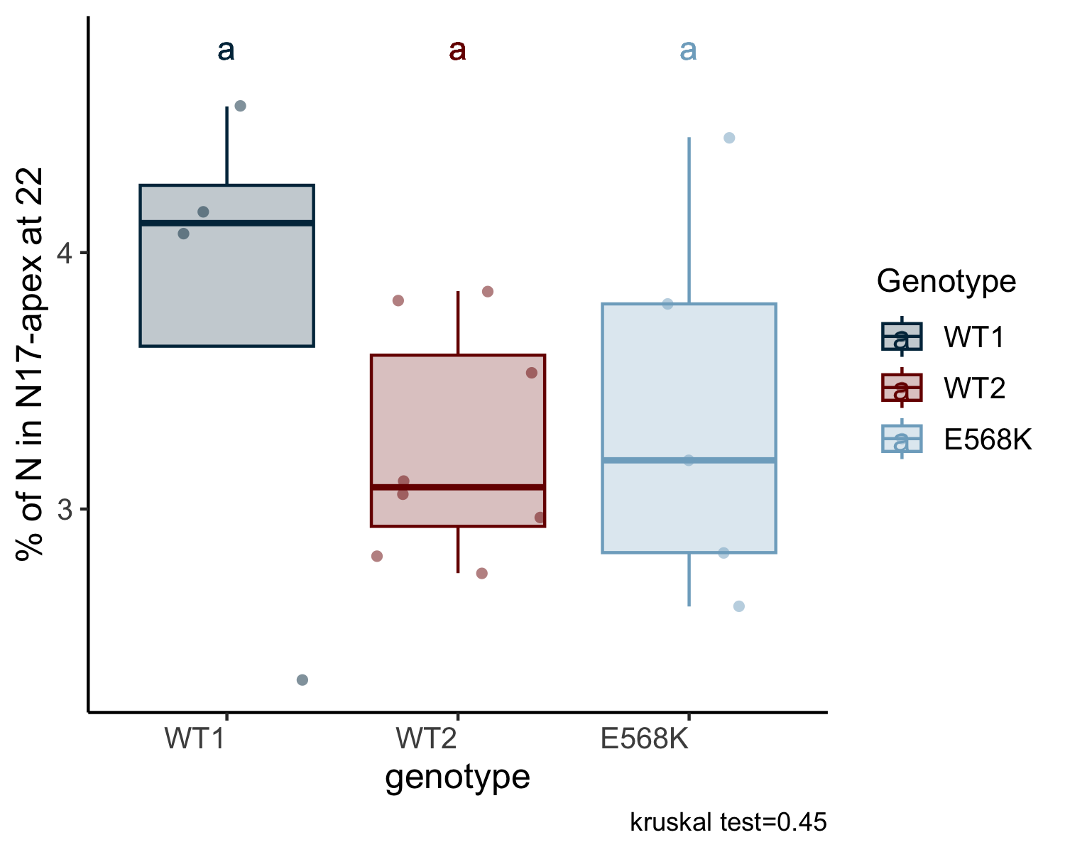
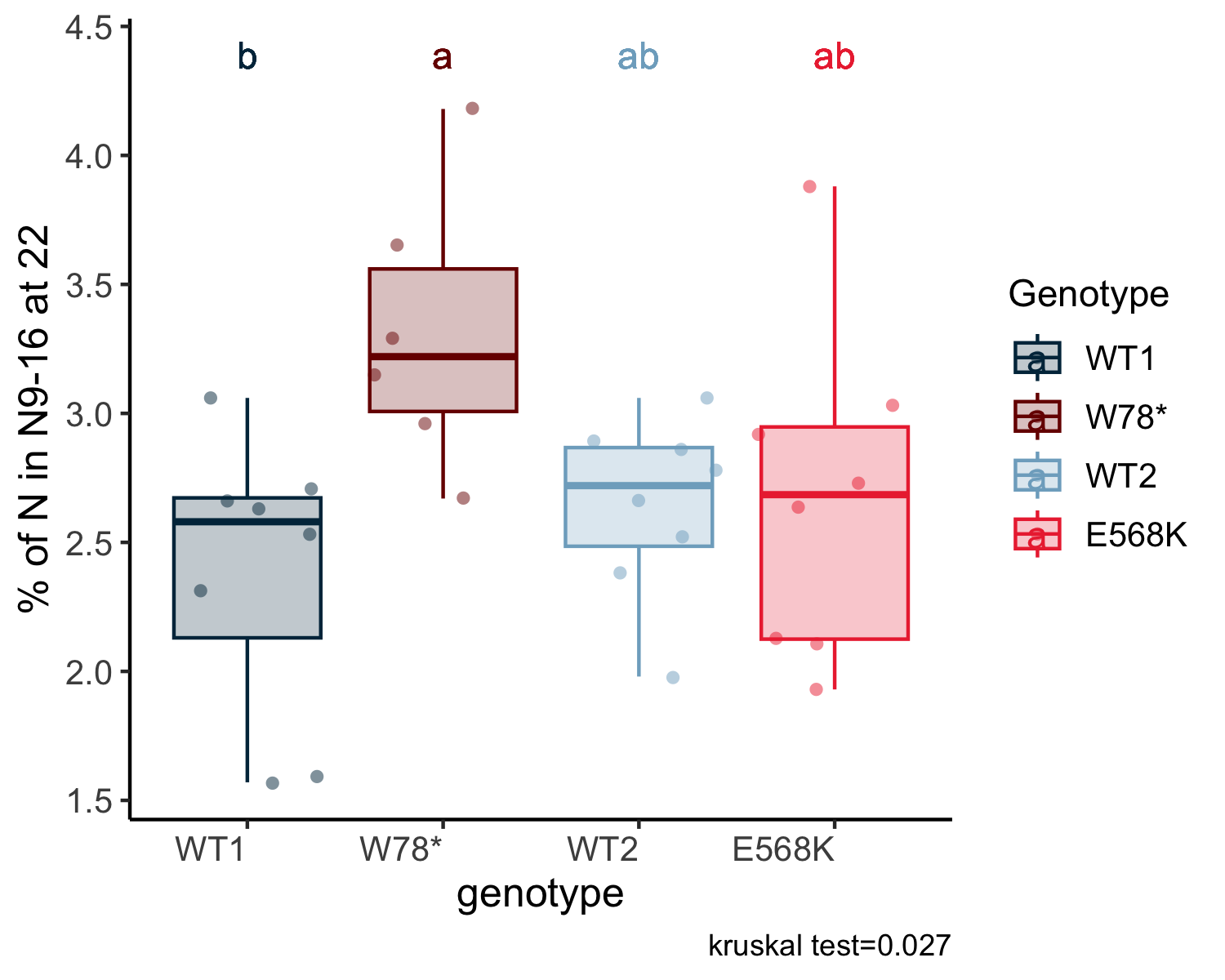
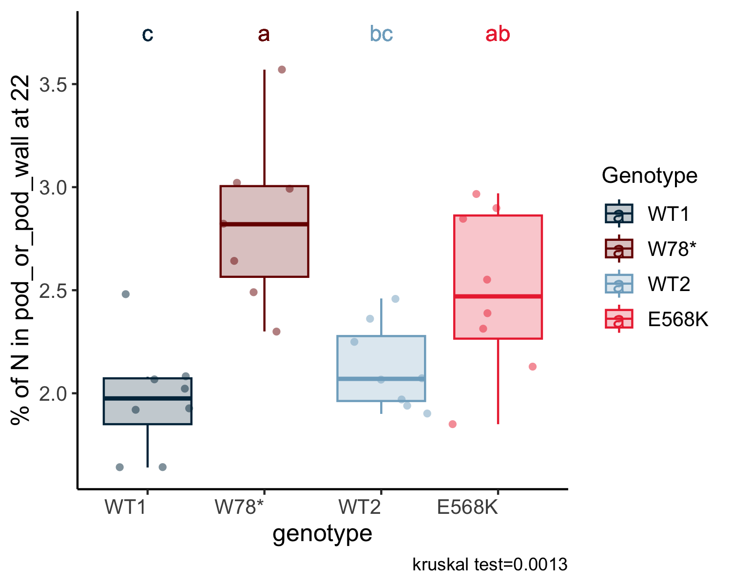
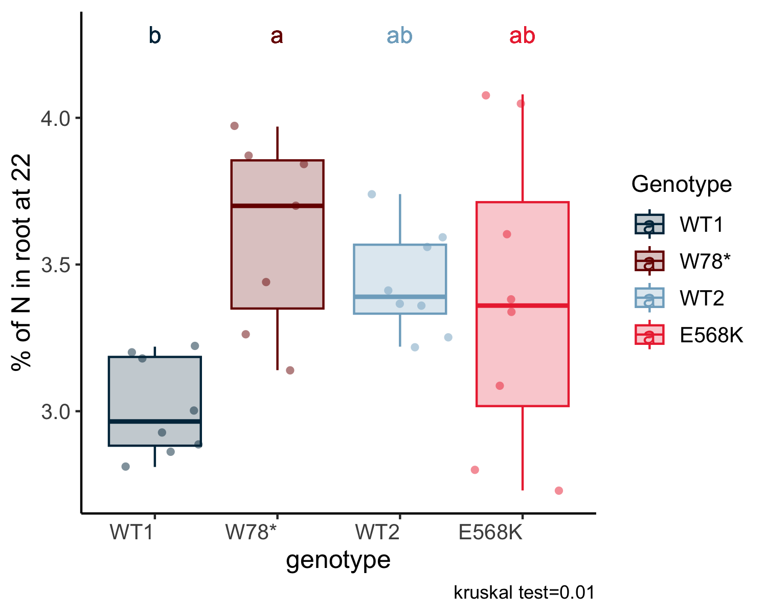
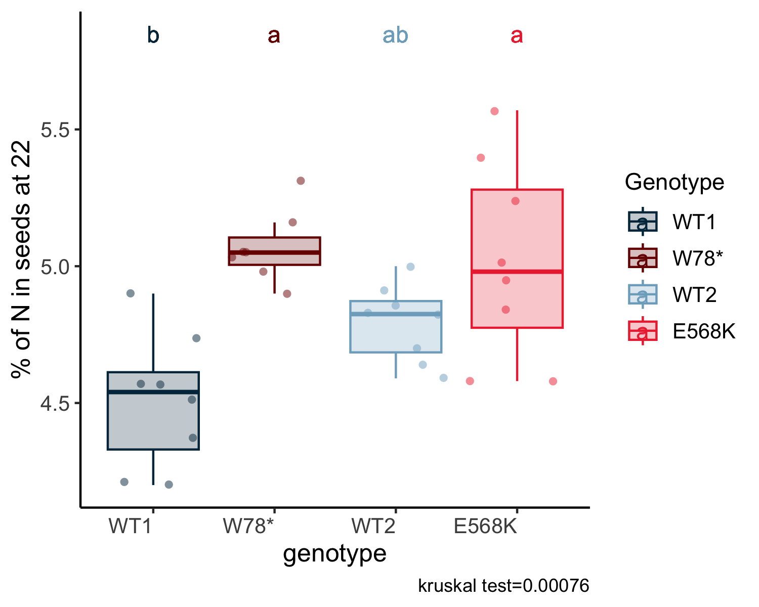
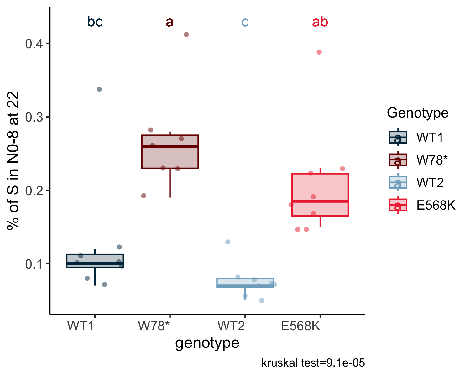
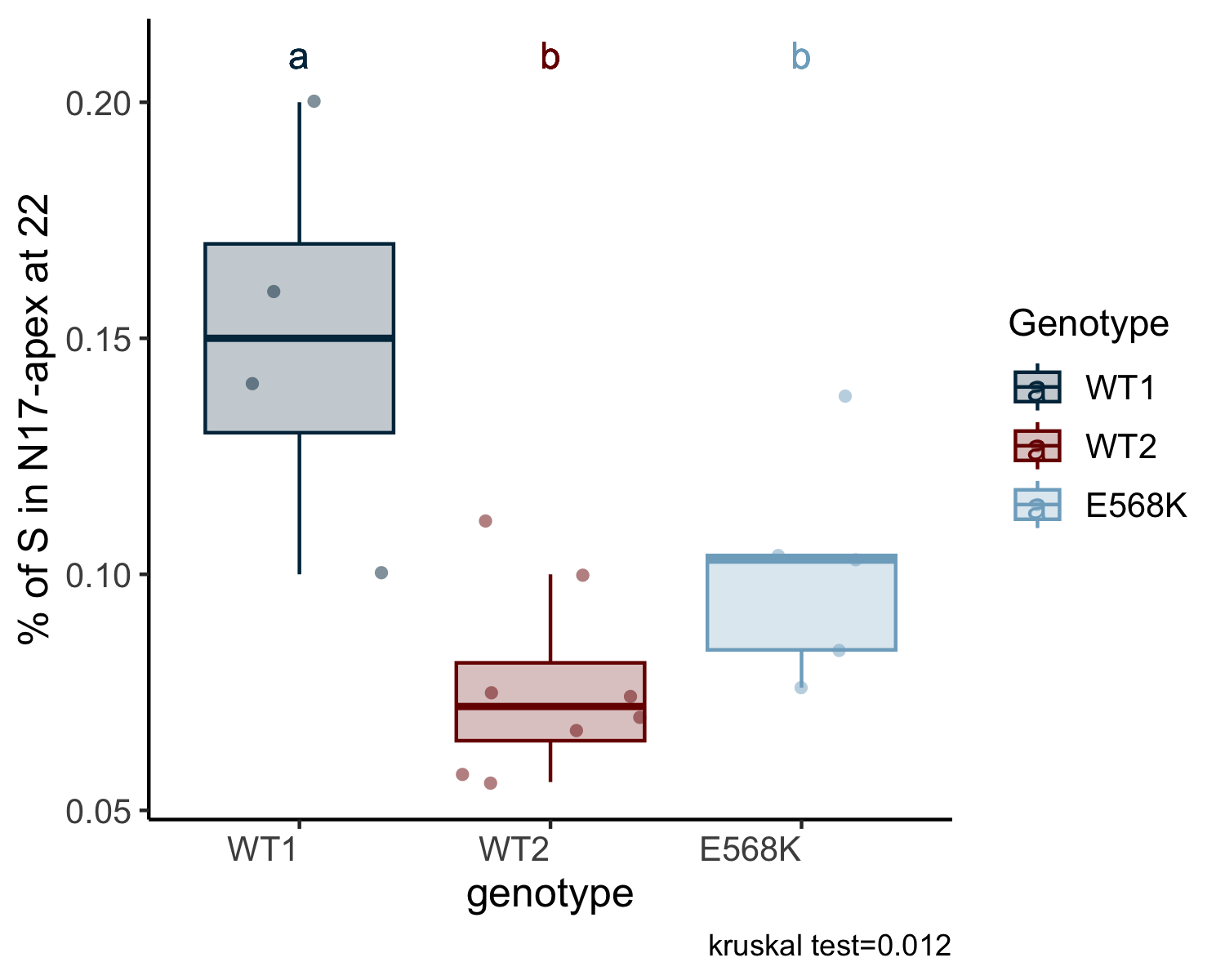
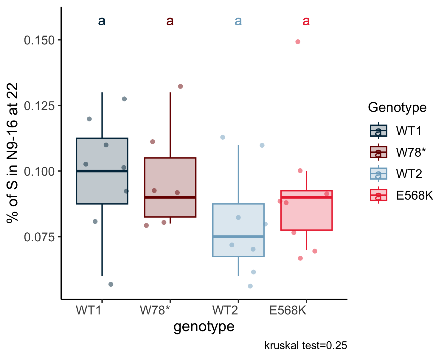
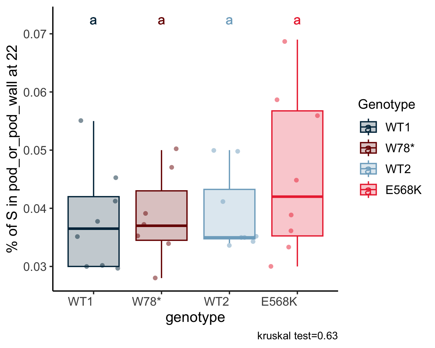
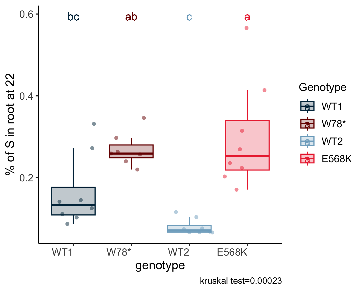
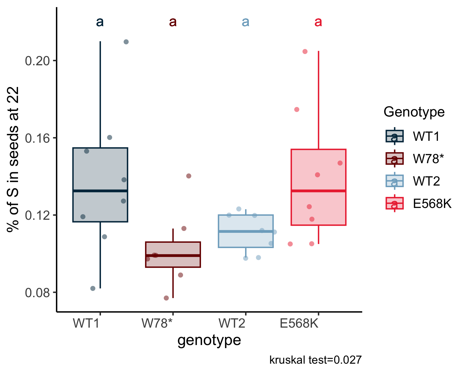
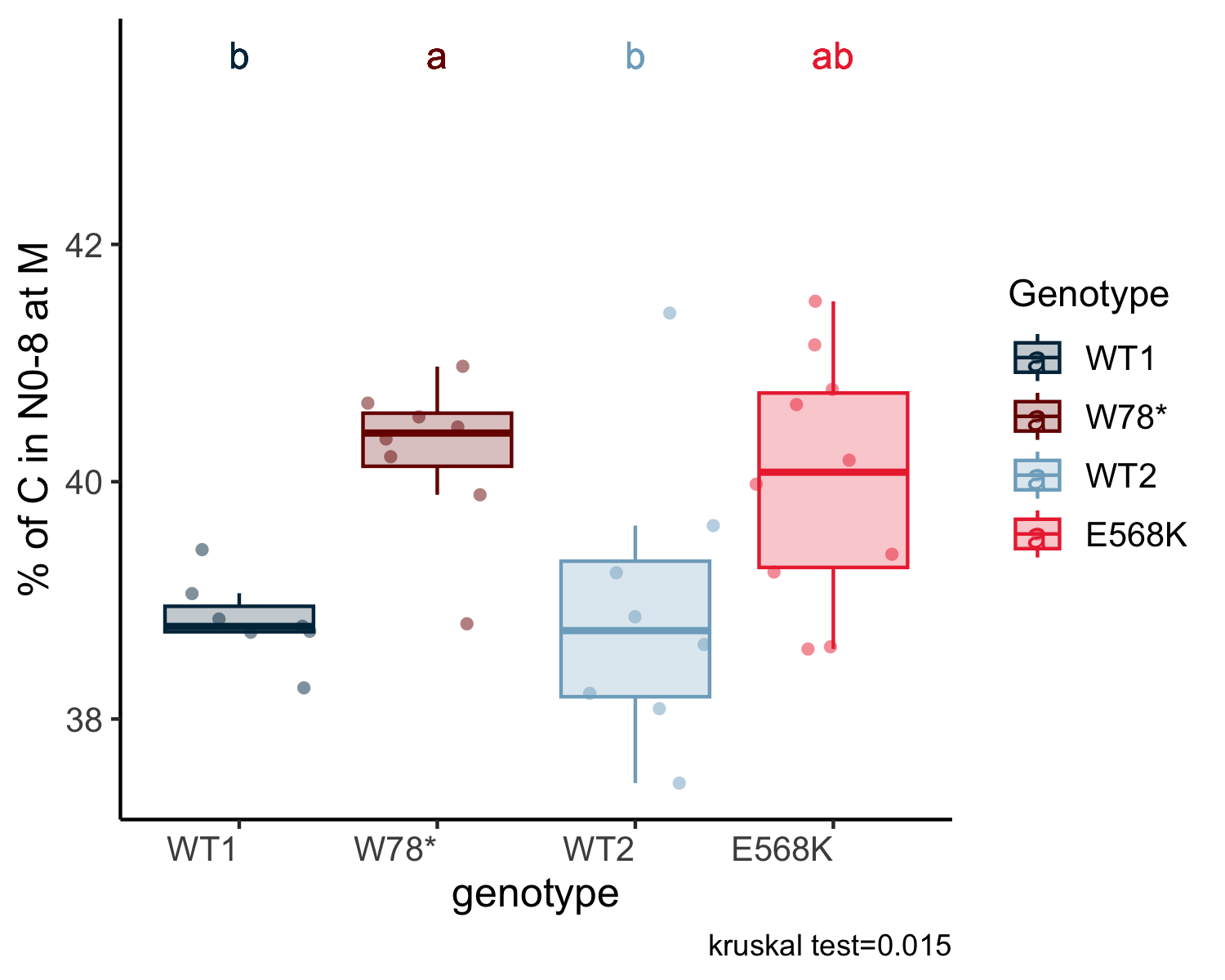
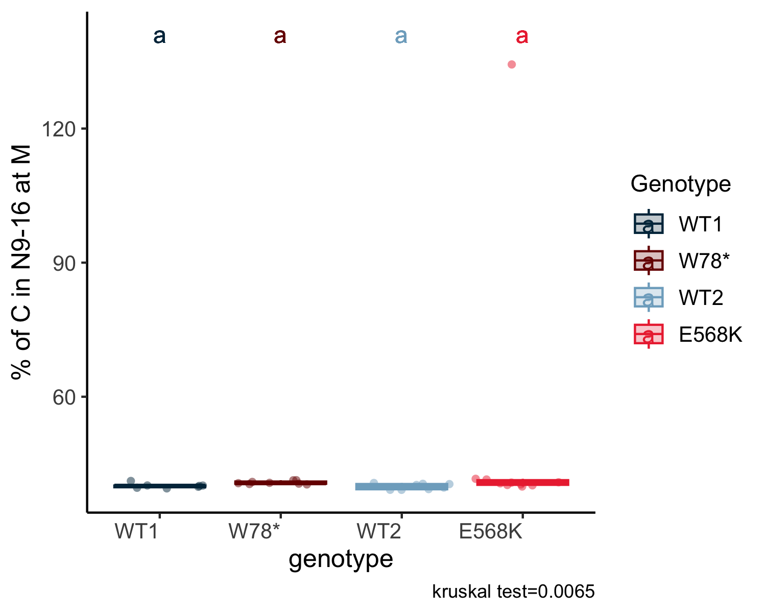
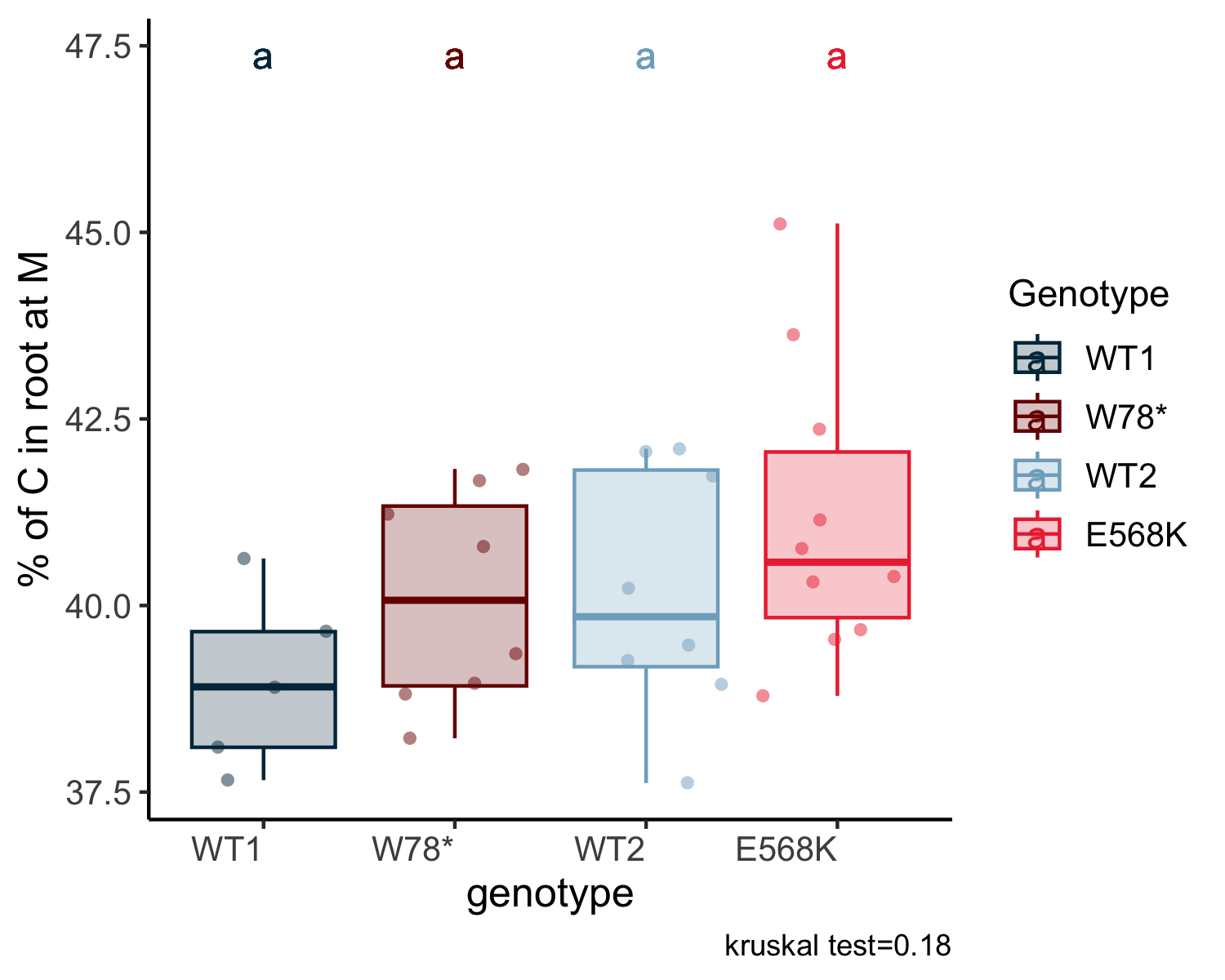
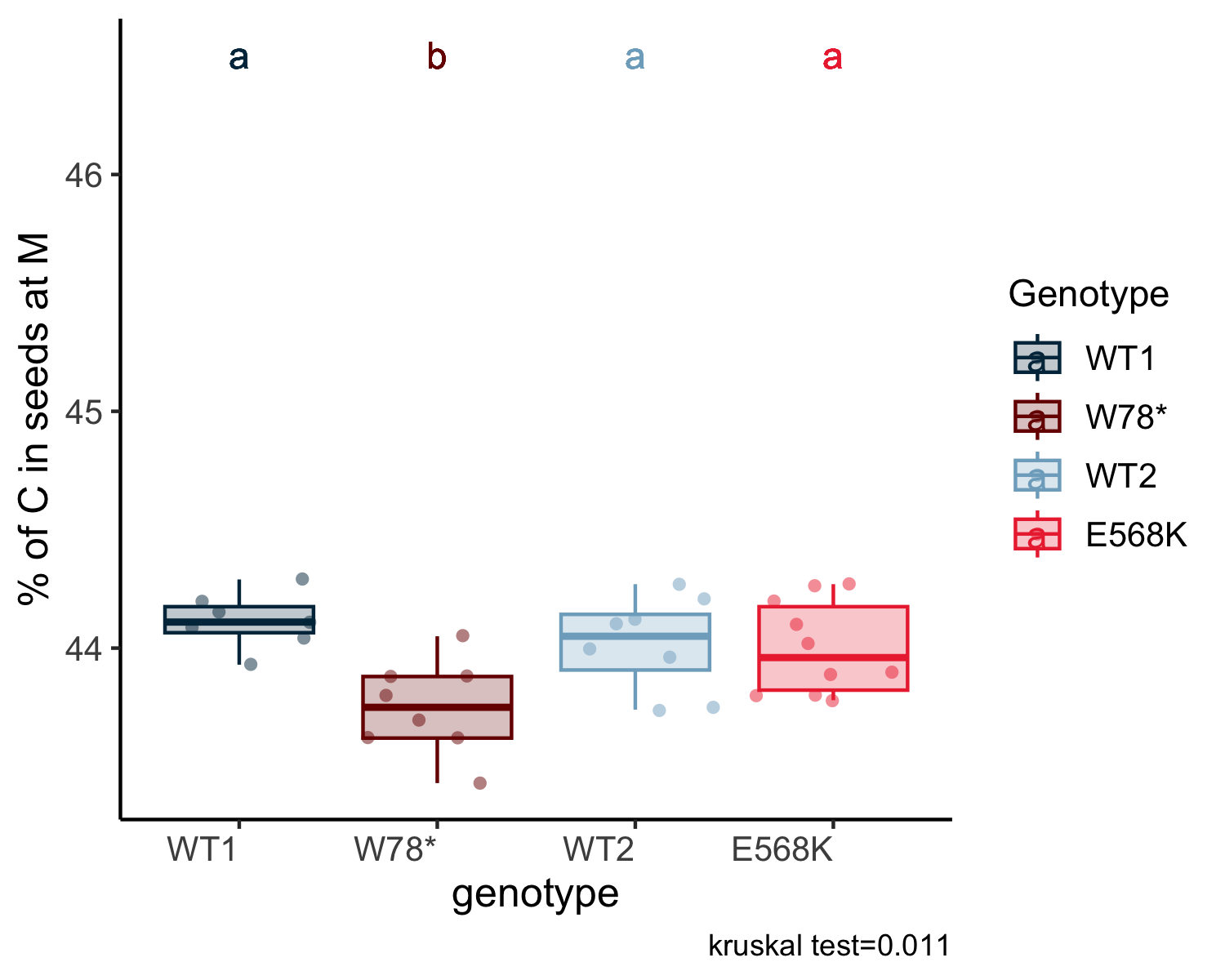
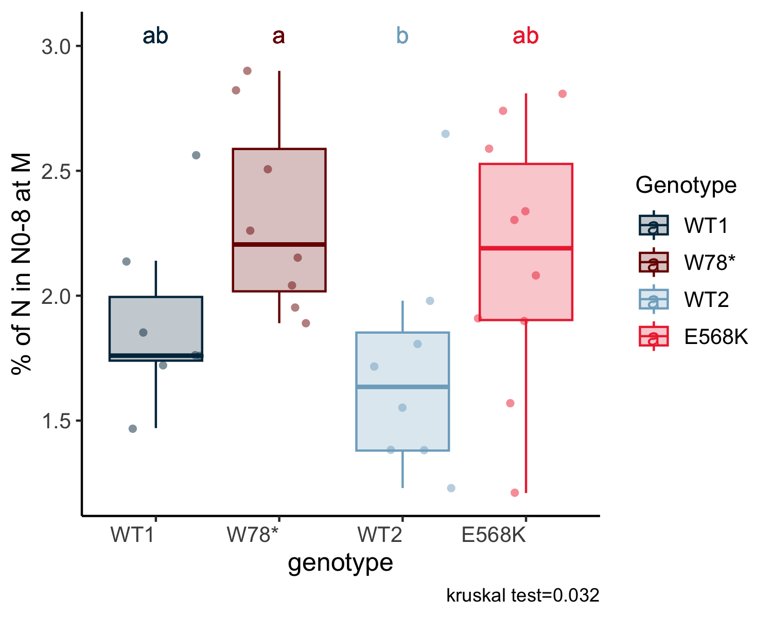
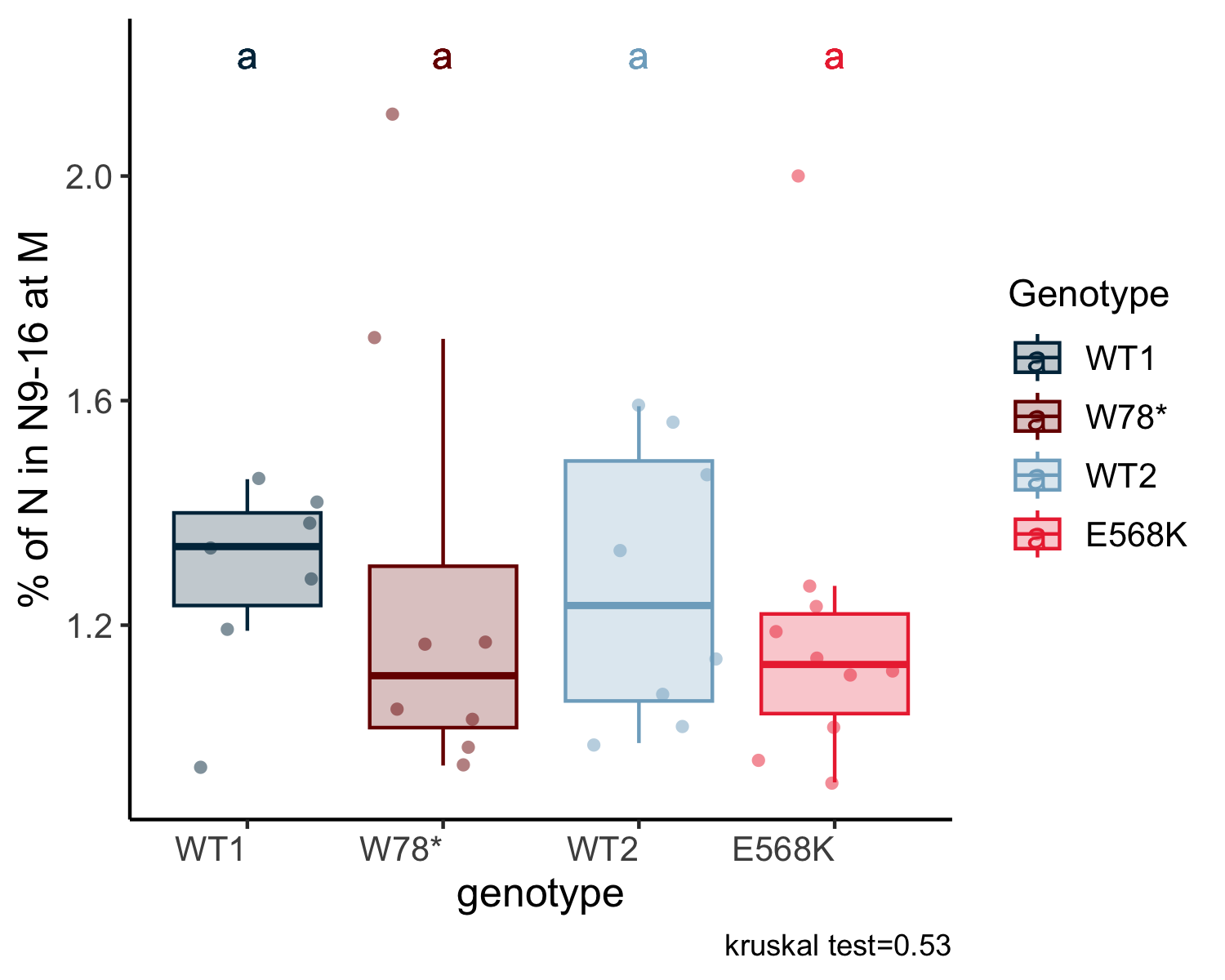
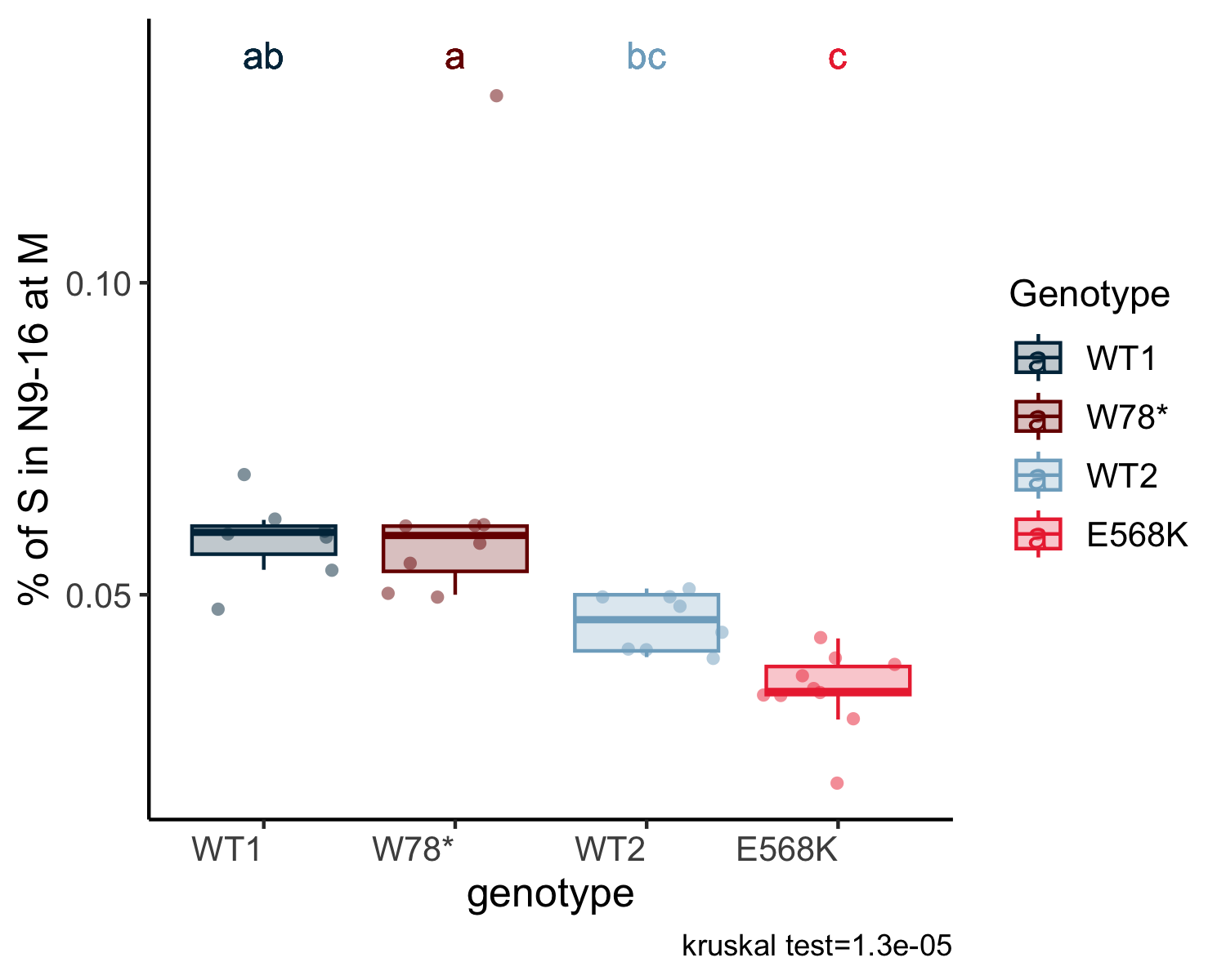
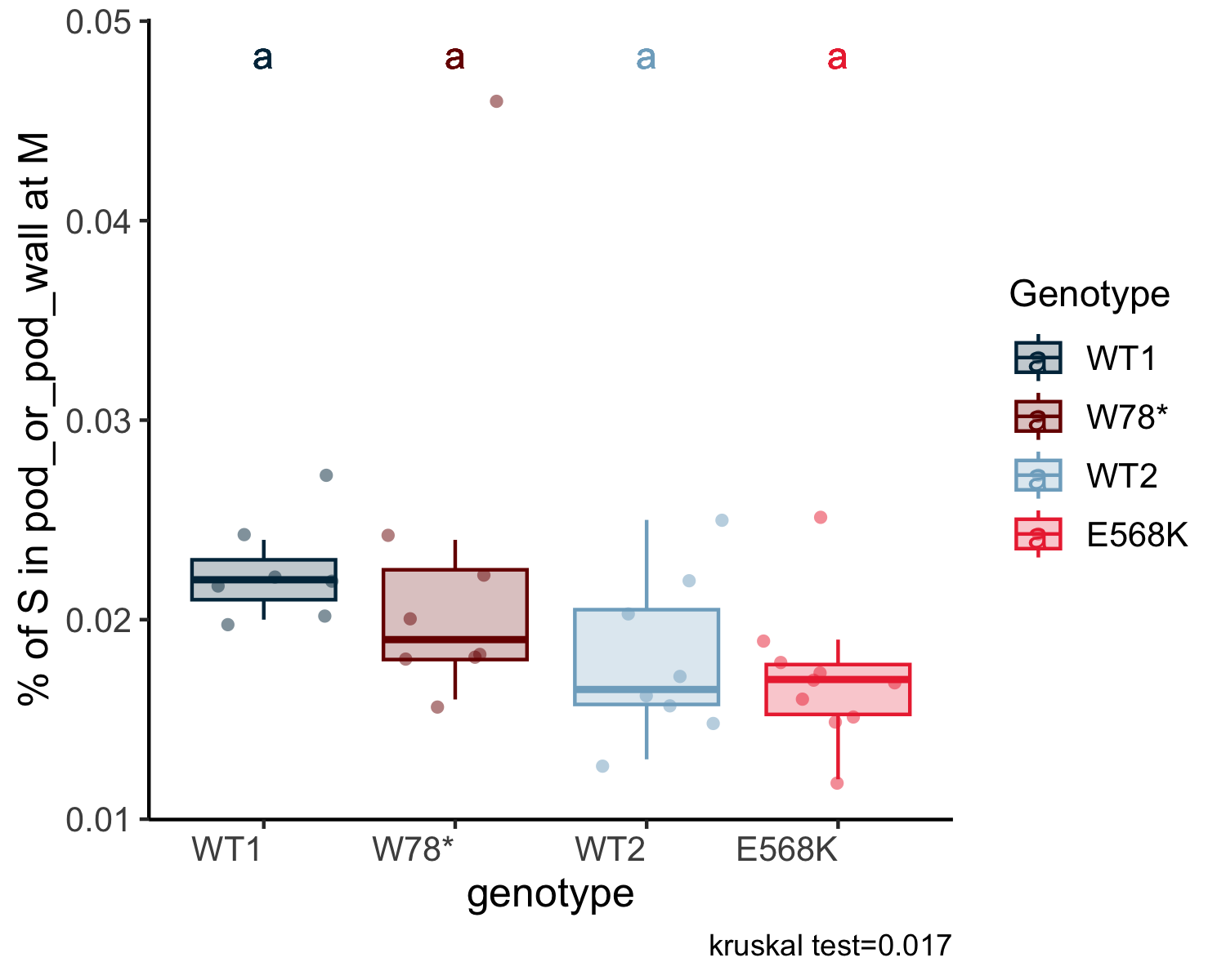
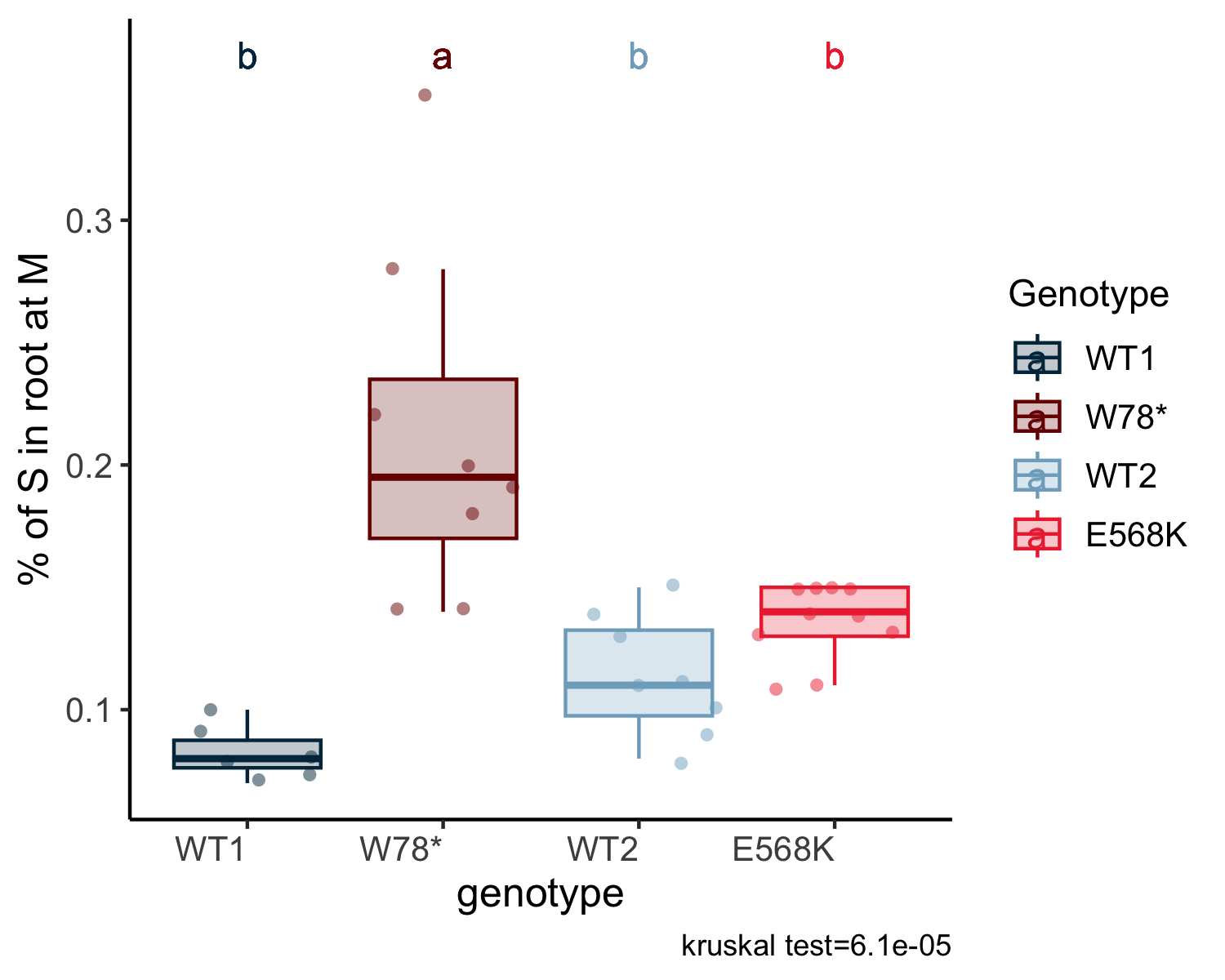
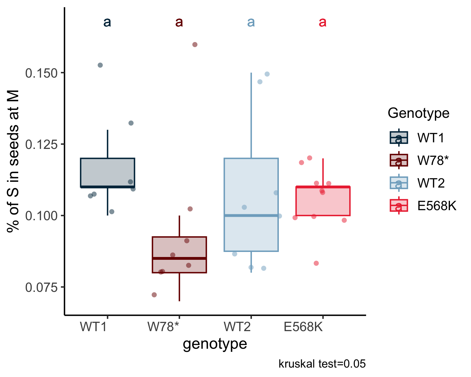
#pkglibrary(readxl)library(tidyverse)library(dplyr)library(ggnewscale) # to have two scale_filllibrary(patchwork)# srcsource(here::here("src/function/stat_function/stat_analysis_main.R")) # for make plot source(here::here("src/function/fig_export.R")) # This function saves a given plot (plot_x) as both a PDF and a high-resolution PNG file at specified dimensions.# cosmeticssulfate_pallet=read_excel(here::here("data/color_palette.xlsm")) %>%filter(set =="sulfure_condition") %>% dplyr::select(color, treatment) %>%pull(color) %>%setNames(read_excel(here::here("data/color_palette.xlsm")) %>%filter(set =="sulfure_condition") %>%pull(treatment) )
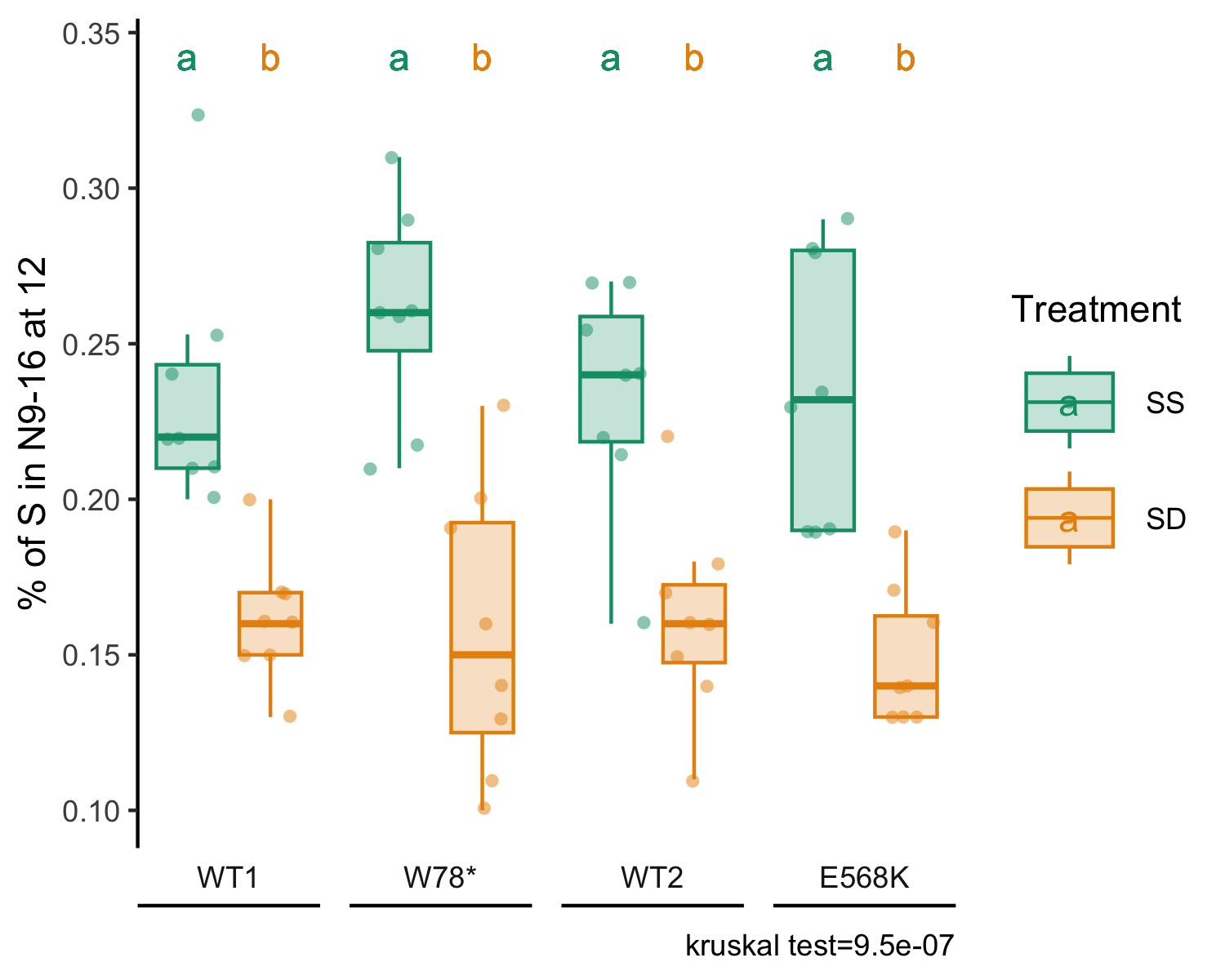
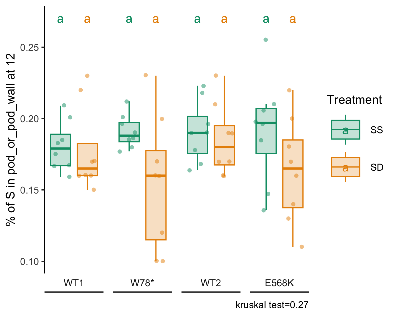
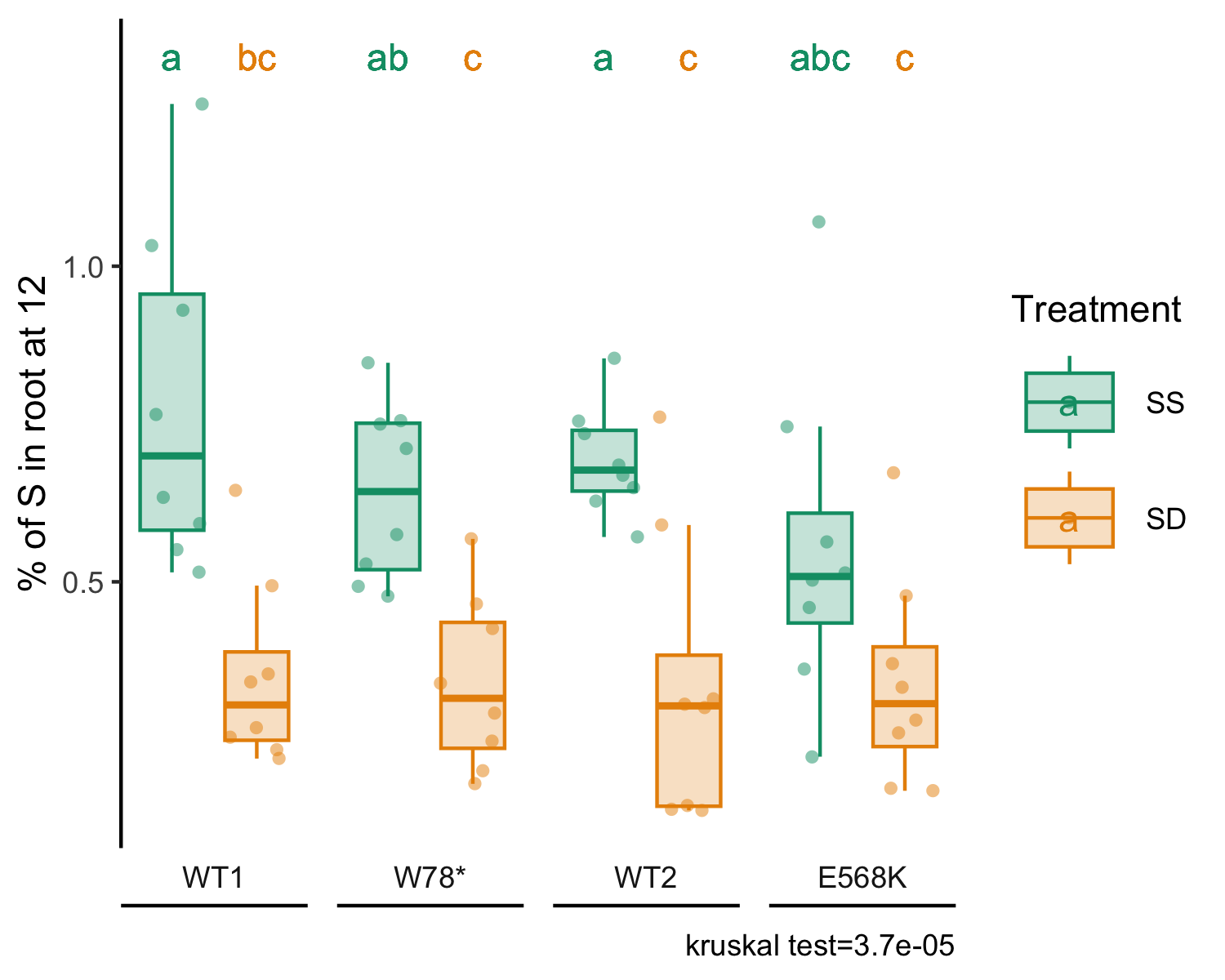
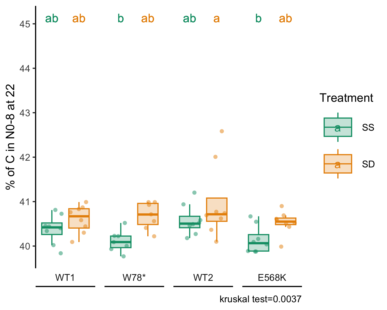
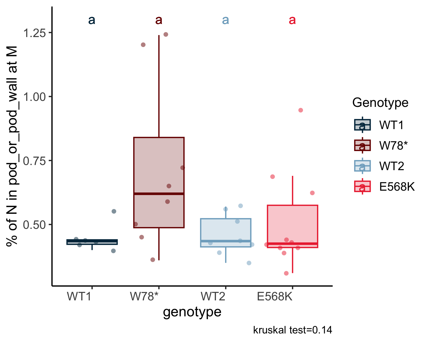
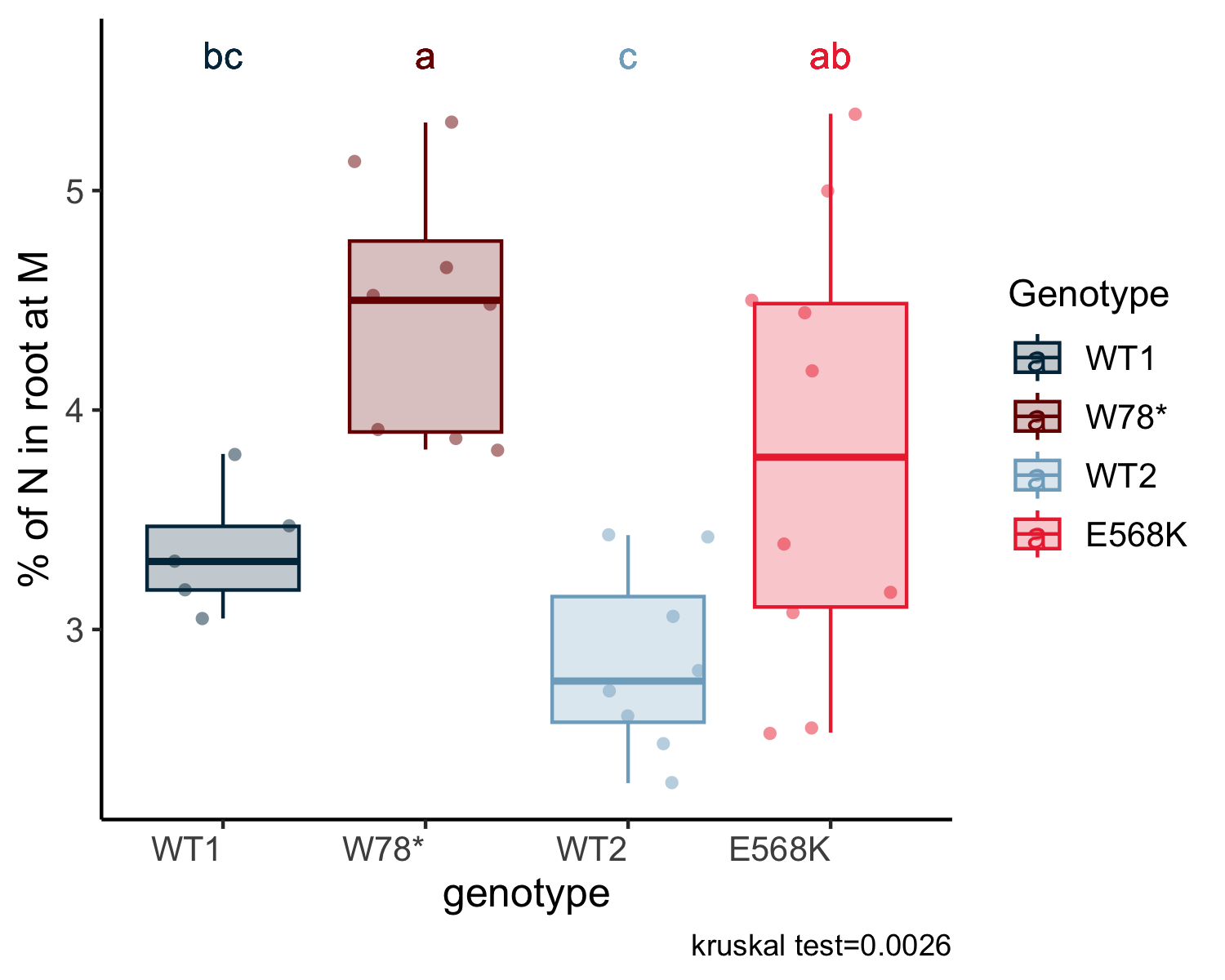
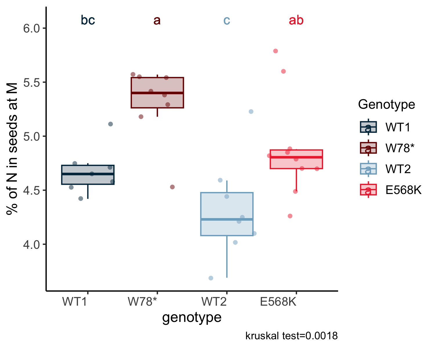
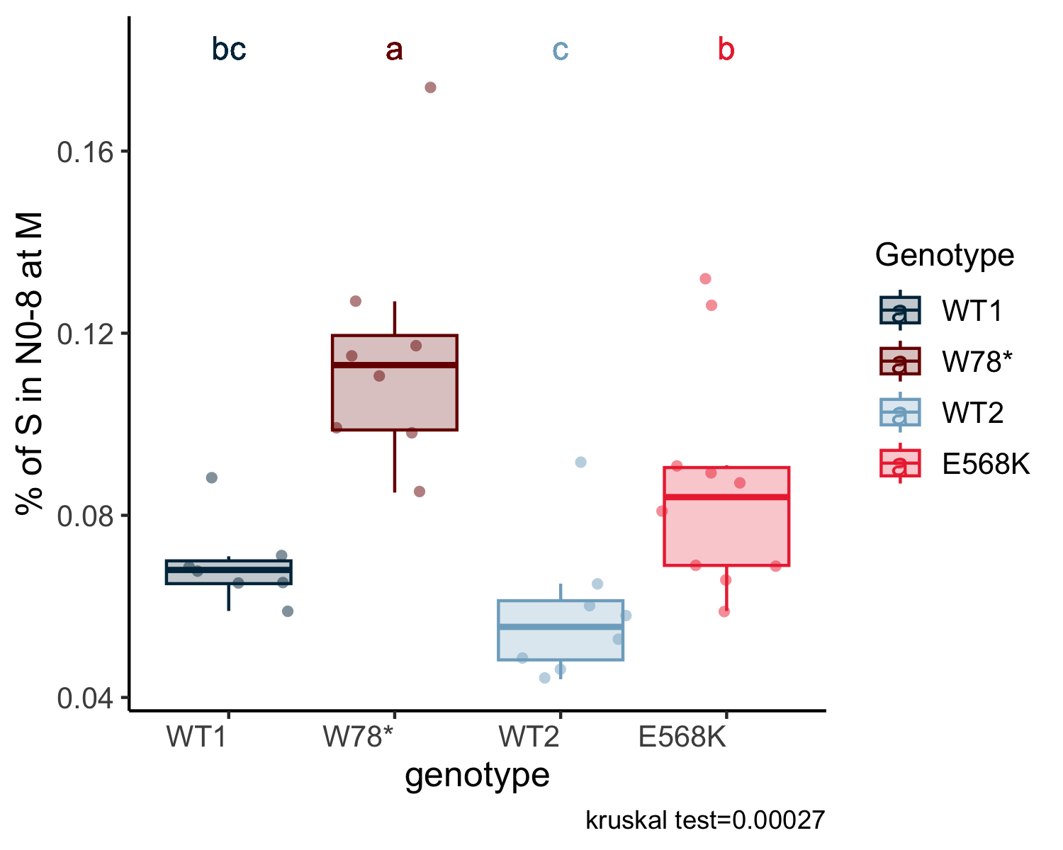
The different compartments of the plants (roots, nodes 1 to 8, nodes 9 to 16 nod 17 to the top; pods and seeds) were separated at different stages (12 days after flowering (DAF) , 22 DAF and at maturity) and their dry weight was determined after oven-drying at 80°C for 48 h, except for dry mature seeds, which were weighed after oven-drying at 30°C for 24 h. S, C and N contents were determined from dried, ground tissue samples from at least six biological replicates using the Dumas method (Allen 1974) on a Carlo Erba elemental analyzer NC2500 (Thermo Fisher Scientific) adapted with a multi-separation column (polytetrafluoroethylene, 2 mm length, internal and external diameters of 5 and 6 mm, respectively; CEElantech ). Prior to analysis, 2 mg vanadium pentoxide was added to 5 mg tissues.
7.1 Data importation
Code
raw_file <-read_excel(here::here("data/CNS/data_pheno_CNS_PO_20140507_V09.xlsx"), sheet ="for_r_importation", col_names = T) %>%mutate(sulfur_condition =ifelse(sulfur_condition =="S+", "SS", "SD")) %>% dplyr::mutate(genotype =case_when( genotype %in%"sultr4;1.1"~"W78*", genotype %in%"sultr4;1.2"~"E568K", genotype %in%"wt.1"~"WT1", genotype %in%"wt.2"~"WT2",TRUE~"Other variable" )) %>%mutate(genotype = forcats::fct_relevel(genotype, "WT1", "W78*", "WT2", "E568K"),condition =paste(sep ="_", genotype, sulfur_condition), sulfur_condition = forcats::fct_relevel(sulfur_condition, "SS", "SD"),stage = forcats::fct_relevel(stage, "Veg", "M", "12", "22"), condition = forcats::fct_relevel(condition, "WT1_SS", "WT1_SD","W78*_SS", "W78*_SD", "WT2_SS", "WT2_SD", "E568K_SS", "E568K_SD") )raw_file_l = raw_file %>%pivot_longer(cols =-c(1:7), names_to ="variable",values_to ="value" )df_element_concentration <- raw_file_l %>%filter(grepl("^(percent_C|percent_N|percent_S)", variable)) %>%separate(variable, into =c("type_variable", "element", "compartment"), sep ="_", extra ="merge")all_possibility <- df_element_concentration %>%distinct(stage, element,compartment)# Initialisation de la liste qui va stocker tous les plotsplots <-list()# Boucle sur chaque combinaisonfor (i inseq_len(nrow(all_possibility))) { stage_i <- all_possibility$stage[i] element_i <- all_possibility$element[i] compartment_i <- all_possibility$compartment[i]# Filtrage des données pour la combinaison courante df_select <- df_element_concentration %>%filter( stage == stage_i, type_variable =="percent", element == element_i, compartment == compartment_i ) %>%drop_na(value) %>%as.data.frame()# Si aucune donnée n'est disponible, on passe à la combinaison suivanteif(nrow(df_select) ==0) {message("Aucune donnée pour: ", stage_i, ", ", element_i, ", ", compartment_i)next }# Définition de l'étiquette de l'axe des ordonnées ylab_i <-paste0("% of ", element_i, " in ", compartment_i, " at ", stage_i)# Essayer d'exécuter stat_analyse et capturer les erreurs éventuelles res <-tryCatch({stat_analyse(data = df_select,column_value ="value",category_variables =c("sulfur_condition"),grp_var ="genotype",show_plot =TRUE,outlier_show =FALSE, label_outlier ="plant_num",biologist_stats =TRUE,Ylab_i = ylab_i,control_conditions =c("SS"),strip_normale =FALSE,hex_pallet = sulfate_pallet ) },error =function(e) {message("Erreur pour: ", stage_i, ", ", element_i, ", ", compartment_i, " -> ", e$message)return(NULL) })# Si une erreur s'est produite, on passe à l'itération suivanteif(is.null(res)) next# Extraction du plot et ajout des labels pour la légende p_plot <- res[["plot"]] +labs(color ="Treatment", fill ="Treatment") plot_name <-paste0(stage_i,"_", element_i, "_", compartment_i)fig_export(here::here(paste0("report/CNS/plot/All_CNS/", plot_name)), p_plot, height_i =4, width_i =5, res_i =300,format ="png") plots[[plot_name]] <- p_plot}# Assemblage de tous les plots avec patchworkfinal_plot <-wrap_plots(plots, ncol =6) +plot_layout(guides ="collect") +plot_annotation() &theme(legend.position ='bottom')# Affichage du plot finalprint(final_plot)fig_export(here::here("report/CNS/plot/all_CNS_stats"), final_plot, height_i =21, width_i =29.7, res_i =600)# R = root ; Nx = nodes(. = to) ; Veg = vegetative nodes ; P = pod (including seeds) ; PW = pod wall ; S = seeds##### only for SD ##### all_possibility <- df_element_concentration %>%filter (sulfur_condition =="SD") %>%distinct(stage, element,compartment)plots <-list()# Boucle sur chaque combinaisonfor (i inseq_len(nrow(all_possibility))) { stage_i <- all_possibility$stage[i] element_i <- all_possibility$element[i] compartment_i <- all_possibility$compartment[i]# Filtrage des données pour la combinaison courante df_select <- df_element_concentration %>%filter( stage == stage_i, type_variable =="percent", element == element_i, compartment == compartment_i ) %>%filter(sulfur_condition =="SD") %>%drop_na(value) %>%as.data.frame()# Si aucune donnée n'est disponible, on passe à la combinaison suivanteif(nrow(df_select) ==0) {message("Aucune donnée pour: ", stage_i, ", ", element_i, ", ", compartment_i)next }# Définition de l'étiquette de l'axe des ordonnées ylab_i <-paste0("% of ", element_i, " in ", compartment_i, " at ", stage_i)# Essayer d'exécuter stat_analyse et capturer les erreurs éventuelles res <-tryCatch({stat_analyse(data = df_select,column_value ="value",category_variables =c("genotype"),grp_var ="",show_plot =TRUE,outlier_show =FALSE, label_outlier ="plant_num",biologist_stats =TRUE,Ylab_i = ylab_i,control_conditions ="",strip_normale =FALSE,hex_pallet =c("#003049", "#780000", "#7FACC7", "#EC323E") ) },error =function(e) {message("Erreur pour: ", stage_i, ", ", element_i, ", ", compartment_i, " -> ", e$message)return(NULL) })# Si une erreur s'est produite, on passe à l'itération suivanteif(is.null(res)) next# Extraction du plot et ajout des labels pour la légende p_plot <- res[["plot"]] +labs(color ="Genotype", fill ="Genotype") plot_name <-paste0(stage_i,"_", element_i,"_", compartment_i)fig_export(here::here(paste0("report/CNS/plot/SD_CNS/", plot_name)), p_plot, height_i =4, width_i =5, res_i =300,format ="png")# Stockage du plot dans la liste avec un nom unique plots[[plot_name]] <- p_plot}# Assemblage de tous les plots avec patchworkfinal_plot <-wrap_plots(plots, ncol =6) +plot_layout(guides ="collect") +plot_annotation() &theme(legend.position ='bottom')# Affichage du plot finalprint(final_plot)fig_export(here::here("report/CNS/plot/SD_CNS_stats"), final_plot, height_i =28, width_i =18, res_i =600)
Allen, David M. 1974. “The Relationship Between Variable Selection and Data Agumentation and a Method for Prediction.”Technometrics 16 (1): 125–27. https://doi.org/10.1080/00401706.1974.10489157.
Source Code
---output: html_documenteditor_options: chunk_output_type: console---## CNS analysis```{r}#pkglibrary(readxl)library(tidyverse)library(dplyr)library(ggnewscale) # to have two scale_filllibrary(patchwork)# srcsource(here::here("src/function/stat_function/stat_analysis_main.R")) # for make plot source(here::here("src/function/fig_export.R")) # This function saves a given plot (plot_x) as both a PDF and a high-resolution PNG file at specified dimensions.# cosmeticssulfate_pallet=read_excel(here::here("data/color_palette.xlsm")) %>%filter(set =="sulfure_condition") %>% dplyr::select(color, treatment) %>%pull(color) %>%setNames(read_excel(here::here("data/color_palette.xlsm")) %>%filter(set =="sulfure_condition") %>%pull(treatment) )```The different compartments of the plants (roots, nodes 1 to 8, nodes 9 to 16 nod 17 to the top; pods and seeds) were separated at different stages (12 days after flowering (DAF) , 22 DAF and at maturity) and their dry weight was determined after oven-drying at 80°C for 48 h, except for dry mature seeds, which were weighed after oven-drying at 30°C for 24 h. S, C and N contents were determined from dried, ground tissue samples from at least six biological replicates using the Dumas method [@allen_relationship_1974] on a Carlo Erba elemental analyzer NC2500 (Thermo Fisher Scientific) adapted with a multi-separation column (polytetrafluoroethylene, 2 mm length, internal and external diameters of 5 and 6 mm, respectively; CE[ Elantech](https://www.ceelantech.com/) ). Prior to analysis, 2 mg vanadium pentoxide was added to 5 mg tissues.## Data importation```{r, eval =F}raw_file <- read_excel(here::here("data/CNS/data_pheno_CNS_PO_20140507_V09.xlsx"), sheet = "for_r_importation", col_names = T) %>% mutate(sulfur_condition = ifelse(sulfur_condition == "S+", "SS", "SD")) %>% dplyr::mutate(genotype = case_when( genotype %in% "sultr4;1.1" ~ "W78*", genotype %in% "sultr4;1.2" ~ "E568K", genotype %in% "wt.1" ~ "WT1", genotype %in% "wt.2" ~ "WT2", TRUE ~ "Other variable" )) %>% mutate(genotype = forcats::fct_relevel(genotype, "WT1", "W78*", "WT2", "E568K"), condition = paste(sep = "_", genotype, sulfur_condition), sulfur_condition = forcats::fct_relevel(sulfur_condition, "SS", "SD"), stage = forcats::fct_relevel(stage, "Veg", "M", "12", "22"), condition = forcats::fct_relevel(condition, "WT1_SS", "WT1_SD", "W78*_SS", "W78*_SD", "WT2_SS", "WT2_SD", "E568K_SS", "E568K_SD") )raw_file_l = raw_file %>% pivot_longer( cols = -c(1:7), names_to = "variable", values_to = "value" )df_element_concentration <- raw_file_l %>% filter(grepl("^(percent_C|percent_N|percent_S)", variable)) %>% separate(variable, into = c("type_variable", "element", "compartment"), sep = "_", extra = "merge")all_possibility <- df_element_concentration %>% distinct(stage, element,compartment)# Initialisation de la liste qui va stocker tous les plotsplots <- list()# Boucle sur chaque combinaisonfor (i in seq_len(nrow(all_possibility))) { stage_i <- all_possibility$stage[i] element_i <- all_possibility$element[i] compartment_i <- all_possibility$compartment[i] # Filtrage des données pour la combinaison courante df_select <- df_element_concentration %>% filter( stage == stage_i, type_variable == "percent", element == element_i, compartment == compartment_i ) %>% drop_na(value) %>% as.data.frame() # Si aucune donnée n'est disponible, on passe à la combinaison suivante if(nrow(df_select) == 0) { message("Aucune donnée pour: ", stage_i, ", ", element_i, ", ", compartment_i) next } # Définition de l'étiquette de l'axe des ordonnées ylab_i <- paste0("% of ", element_i, " in ", compartment_i, " at ", stage_i) # Essayer d'exécuter stat_analyse et capturer les erreurs éventuelles res <- tryCatch({ stat_analyse( data = df_select, column_value = "value", category_variables = c("sulfur_condition"), grp_var = "genotype", show_plot = TRUE, outlier_show = FALSE, label_outlier = "plant_num", biologist_stats = TRUE, Ylab_i = ylab_i, control_conditions = c("SS"), strip_normale = FALSE, hex_pallet = sulfate_pallet ) }, error = function(e) { message("Erreur pour: ", stage_i, ", ", element_i, ", ", compartment_i, " -> ", e$message) return(NULL) }) # Si une erreur s'est produite, on passe à l'itération suivante if(is.null(res)) next # Extraction du plot et ajout des labels pour la légende p_plot <- res[["plot"]] + labs(color = "Treatment", fill = "Treatment") plot_name <- paste0(stage_i,"_", element_i, "_", compartment_i) fig_export(here::here(paste0("report/CNS/plot/All_CNS/", plot_name)), p_plot, height_i = 4, width_i = 5, res_i = 300,format = "png") plots[[plot_name]] <- p_plot}# Assemblage de tous les plots avec patchworkfinal_plot <- wrap_plots(plots, ncol = 6) + plot_layout(guides = "collect") + plot_annotation() & theme(legend.position = 'bottom')# Affichage du plot finalprint(final_plot)fig_export(here::here("report/CNS/plot/all_CNS_stats"), final_plot, height_i = 21, width_i = 29.7, res_i = 600)# R = root ; Nx = nodes(. = to) ; Veg = vegetative nodes ; P = pod (including seeds) ; PW = pod wall ; S = seeds##### only for SD ##### all_possibility <- df_element_concentration %>% filter (sulfur_condition == "SD") %>% distinct(stage, element,compartment)plots <- list()# Boucle sur chaque combinaisonfor (i in seq_len(nrow(all_possibility))) { stage_i <- all_possibility$stage[i] element_i <- all_possibility$element[i] compartment_i <- all_possibility$compartment[i] # Filtrage des données pour la combinaison courante df_select <- df_element_concentration %>% filter( stage == stage_i, type_variable == "percent", element == element_i, compartment == compartment_i ) %>% filter(sulfur_condition == "SD") %>% drop_na(value) %>% as.data.frame() # Si aucune donnée n'est disponible, on passe à la combinaison suivante if(nrow(df_select) == 0) { message("Aucune donnée pour: ", stage_i, ", ", element_i, ", ", compartment_i) next } # Définition de l'étiquette de l'axe des ordonnées ylab_i <- paste0("% of ", element_i, " in ", compartment_i, " at ", stage_i) # Essayer d'exécuter stat_analyse et capturer les erreurs éventuelles res <- tryCatch({ stat_analyse( data = df_select, column_value = "value", category_variables = c("genotype"), grp_var = "", show_plot = TRUE, outlier_show = FALSE, label_outlier = "plant_num", biologist_stats = TRUE, Ylab_i = ylab_i, control_conditions = "", strip_normale = FALSE, hex_pallet = c("#003049", "#780000", "#7FACC7", "#EC323E") ) }, error = function(e) { message("Erreur pour: ", stage_i, ", ", element_i, ", ", compartment_i, " -> ", e$message) return(NULL) }) # Si une erreur s'est produite, on passe à l'itération suivante if(is.null(res)) next # Extraction du plot et ajout des labels pour la légende p_plot <- res[["plot"]] + labs(color = "Genotype", fill = "Genotype") plot_name <- paste0(stage_i,"_", element_i,"_", compartment_i) fig_export(here::here(paste0("report/CNS/plot/SD_CNS/", plot_name)), p_plot, height_i = 4, width_i = 5, res_i = 300,format = "png") # Stockage du plot dans la liste avec un nom unique plots[[plot_name]] <- p_plot}# Assemblage de tous les plots avec patchworkfinal_plot <- wrap_plots(plots, ncol = 6) + plot_layout(guides = "collect") + plot_annotation() & theme(legend.position = 'bottom')# Affichage du plot finalprint(final_plot)fig_export(here::here("report/CNS/plot/SD_CNS_stats"), final_plot, height_i = 28, width_i = 18, res_i = 600)```**For SS and SD**```{r, echo=FALSE, results = "asis"}# Liste des images dans un dossierimage_files <- list.files("plot/CNS/All_CNS", pattern = "\\.png$", full.names = TRUE)# Extraire le nom des fichiers sans extensionimage_names <- tools::file_path_sans_ext(basename(image_files))# Extraire la première et la deuxième valeur séparées par "_"first_values <- sapply(strsplit(image_names, "_"), function(x) x[1])second_values <- sapply(strsplit(image_names, "_"), function(x) x[2])# Identifier les groupes uniques pour la première valeurunique_first <- unique(first_values)# Création du code pour le panel-tabset globaltabset_code <- ":::: {.panel-tabset}\n"# Pour chaque groupe du premier niveaufor (grp1 in unique_first) { tabset_code <- paste0(tabset_code, "## ", grp1, "\n\n", ":::: {.panel-tabset}\n") # Indices des images appartenant à ce groupe indices_first <- which(first_values == grp1) # Identifier les sous-groupes (deuxième valeur) dans ce groupe unique_second <- unique(second_values[indices_first]) # Pour chaque sous-groupe du deuxième niveau for (grp2 in unique_second) { tabset_code <- paste0(tabset_code, "### ", grp2, "\n\n", ":::: {.panel-tabset}\n") # Sélectionner les images correspondant à ce sous-groupe indices_second <- indices_first[second_values[indices_first] == grp2] for (i in indices_second) { tabset_code <- paste0(tabset_code, "#### ", image_names[i], "\n\n", " } tabset_code <- paste0(tabset_code, "::::\n\n") # fermeture du sous-tabset du deuxième niveau } tabset_code <- paste0(tabset_code, "::::\n\n") # fermeture du sous-tabset du premier niveau}tabset_code <- paste0(tabset_code, "::::")cat(tabset_code)```**For SD only**```{r, echo=FALSE, results = "asis"}# Liste des images dans un dossierimage_files <- list.files("plot/CNS/SD_CNS", pattern = "\\.png$", full.names = TRUE)# Extraire le nom des fichiers sans extensionimage_names <- tools::file_path_sans_ext(basename(image_files))# Extraire la première et la deuxième valeur séparées par "_"first_values <- sapply(strsplit(image_names, "_"), function(x) x[1])second_values <- sapply(strsplit(image_names, "_"), function(x) x[2])# Identifier les groupes uniques pour la première valeurunique_first <- unique(first_values)# Création du code pour le panel-tabset globaltabset_code <- ":::: {.panel-tabset}\n"# Pour chaque groupe du premier niveaufor (grp1 in unique_first) { tabset_code <- paste0(tabset_code, "## ", grp1, "\n\n", ":::: {.panel-tabset}\n") # Indices des images appartenant à ce groupe indices_first <- which(first_values == grp1) # Identifier les sous-groupes (deuxième valeur) dans ce groupe unique_second <- unique(second_values[indices_first]) # Pour chaque sous-groupe du deuxième niveau for (grp2 in unique_second) { tabset_code <- paste0(tabset_code, "### ", grp2, "\n\n", ":::: {.panel-tabset}\n") # Sélectionner les images correspondant à ce sous-groupe indices_second <- indices_first[second_values[indices_first] == grp2] for (i in indices_second) { tabset_code <- paste0(tabset_code, "#### ", image_names[i], "\n\n", " } tabset_code <- paste0(tabset_code, "::::\n\n") # fermeture du sous-tabset du deuxième niveau } tabset_code <- paste0(tabset_code, "::::\n\n") # fermeture du sous-tabset du premier niveau}tabset_code <- paste0(tabset_code, "::::")cat(tabset_code)```