6  Plant developpment (2025)

Code
#pkg
library(tidyverse)
library(here)
library(readxl)
library(ggh4x)
library(ggstats)
library(progressr)

# src
source(here::here("src/function/stat_function/stat_analysis_main.R")) # for make plot 
source(here::here("src/function/fig_export.R")) # This function saves a given plot (plot_x) as both a PDF and a high-resolution PNG file at specified dimensions.

# cosmetics
sulfate_pallet=read_excel(here::here("data/color_palette.xlsm")) %>%
      filter(set == "sulfure_condition") %>%
      dplyr::select(color, treatment) %>%
      pull(color) %>%
      setNames(read_excel(here::here("data/color_palette.xlsm")) %>%
                 filter(set == "sulfure_condition") %>%
                 pull(treatment)
               )
mutant_palette=read_excel(here::here("data/color_palette.xlsm")) %>%
      filter(set == "mutant") %>%
      dplyr::select(color, treatment) %>%
      pull(color) %>%
      setNames(read_excel(here::here("data/color_palette.xlsm")) %>%
                 filter(set == "mutant") %>%
                 pull(treatment)
               )

There are 40 plants.

6.1 Data importation

Code
plant_info <- read_excel(here::here("data/plant_info.xlsx"), col_names = T) %>% 
  dplyr::rename("position"= "tablar position")

df_developement <- read_excel(here::here("data/physio/SPAD_greenhouse_2025_raw_data.xlsx"), col_names = T, sheet = "dvt_spad_20250429") %>% 
  drop_na(pod)

write_csv(x = df_developement, file = here::here("data/physio/output/df_development.csv"))

6.2 Quick observation of results

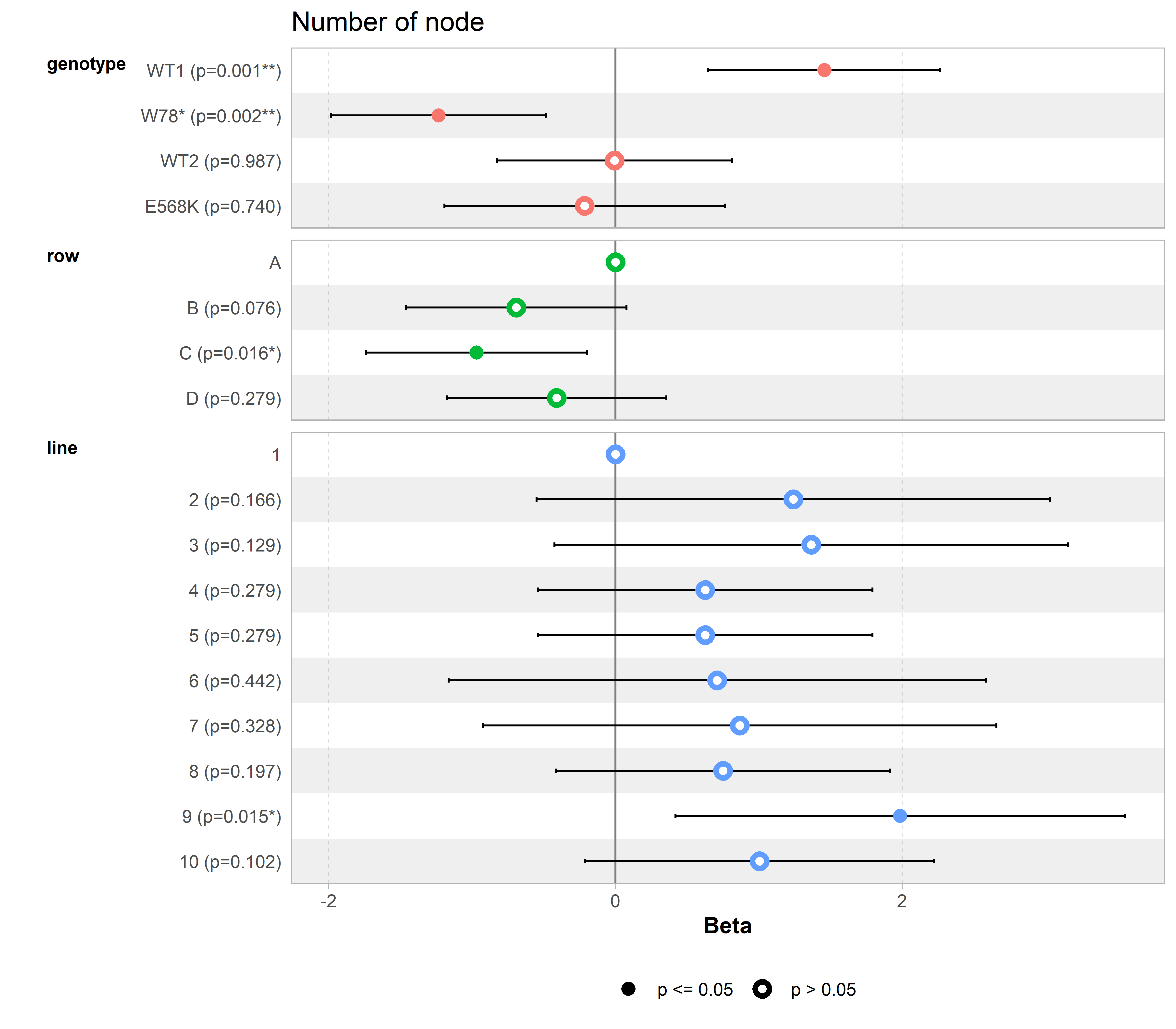
6.2.1 ggcoef

Code
df_development <- read_csv(file = here::here("data/physio/output/df_development.csv"),show_col_types = FALSE ) %>% 
  mutate(plant_num = as.factor(plant_num),
         line = as.factor(line),
         genotype = as.factor(genotype),
         genotype=fct_relevel(genotype, "WT1", "W78*", "WT2", "E568K"), # warning is 8 
         date = as.factor(date))

contrasts(df_development$genotype) <- contr.sum # to say look at the big average only for genotype (juste an other representation)
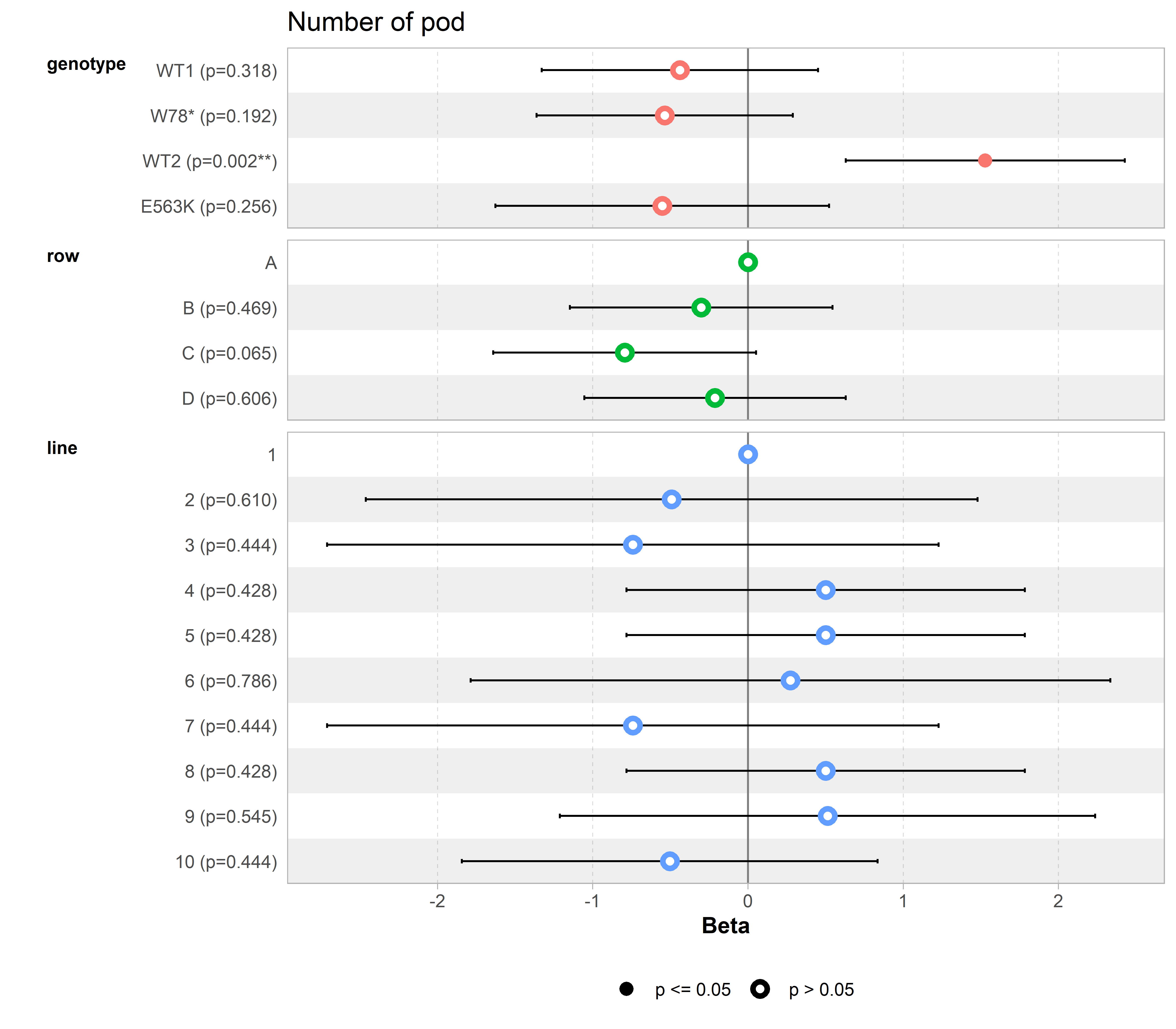
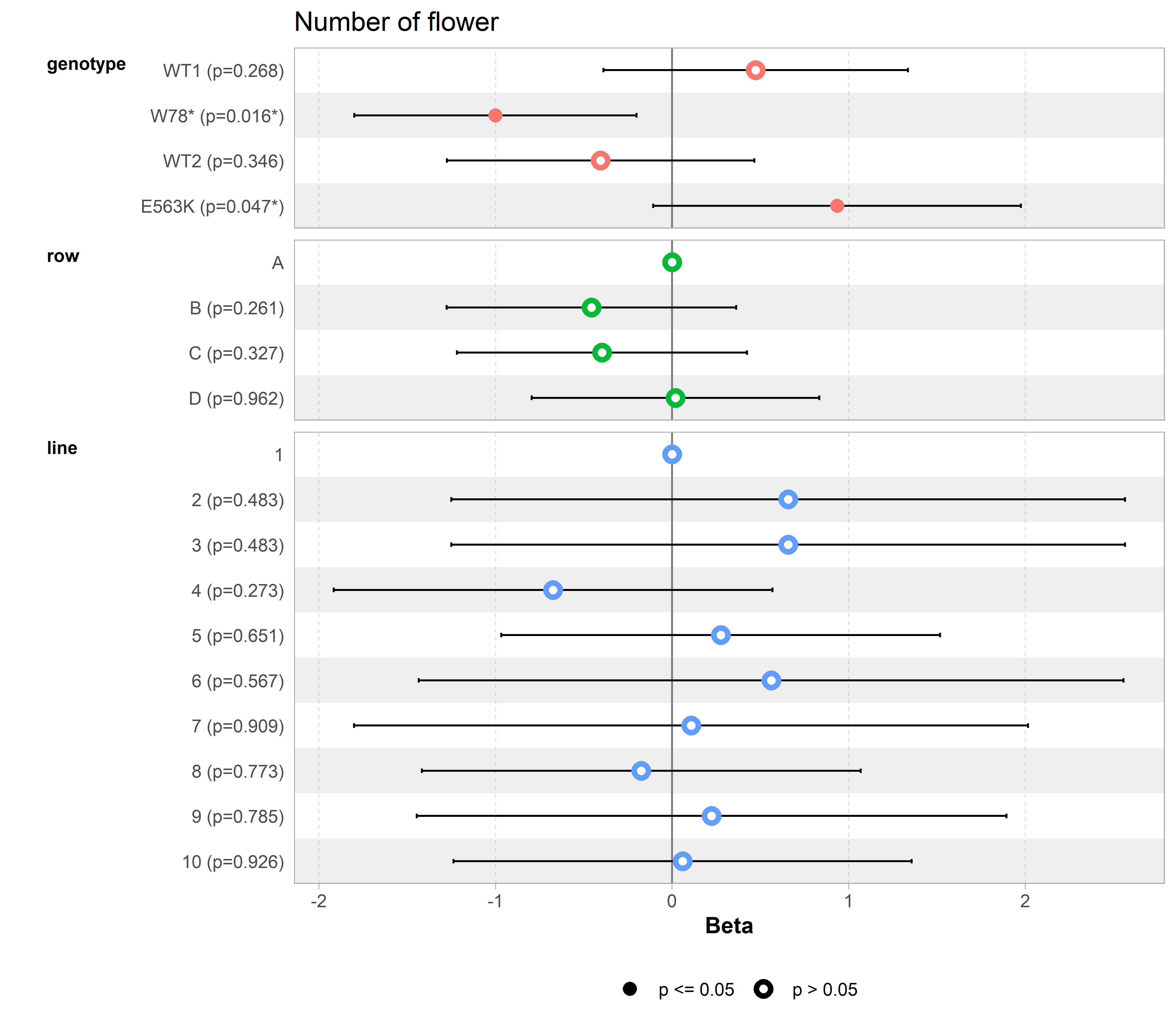
mod1=lm(formula = development ~ genotype+row+line, data = df_development)
p_x<-ggcoef_model(mod1)+
  labs(title = "Number of node")

fig_export(here::here("report/physio/plot/development/ggcoef_model_development"), p_x, height_i = 7, width_i = 8, res_i = 600)

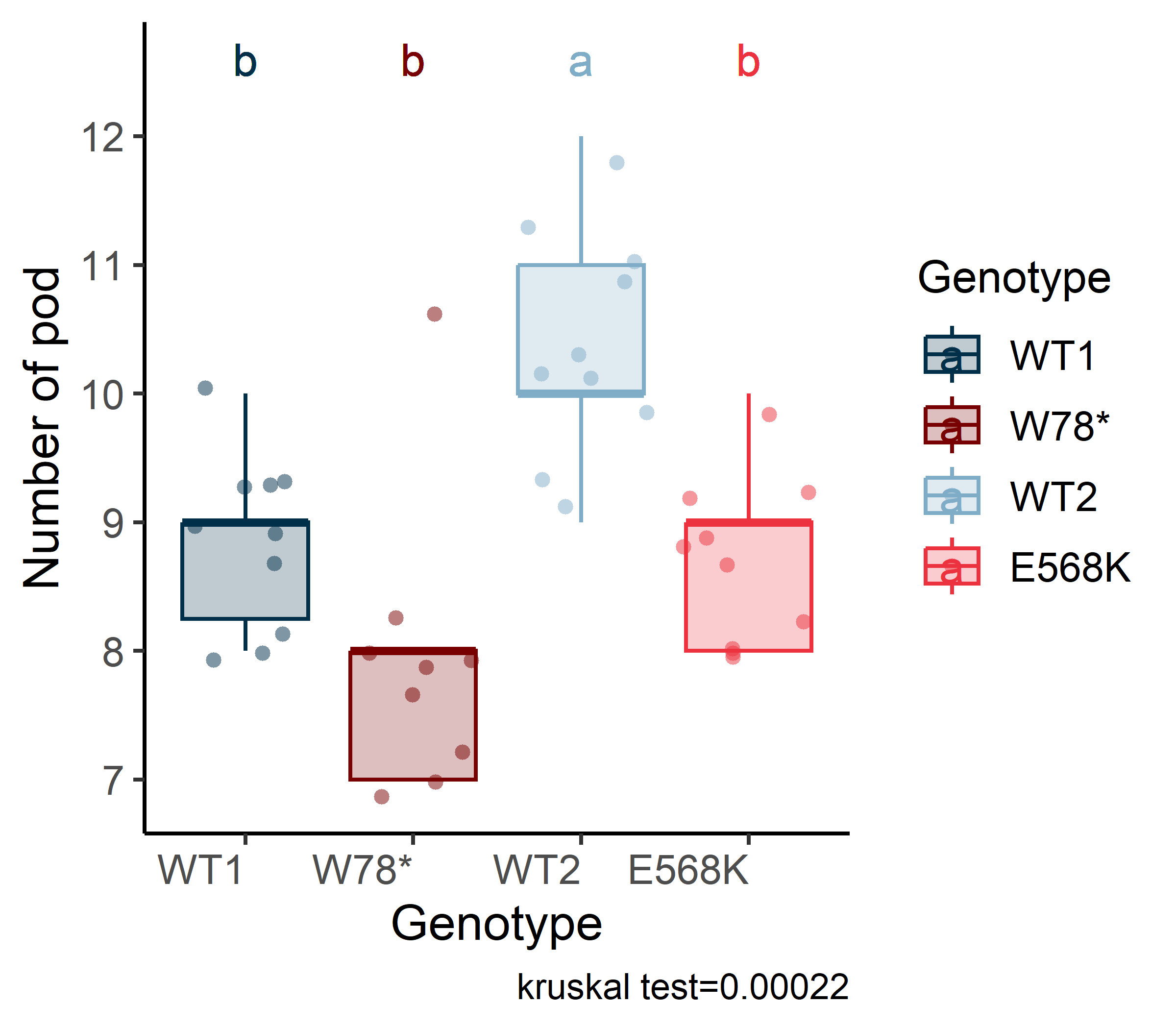
6.2.2 Plot Stats

Code
df_development <- read_csv(file = here::here("data/physio/output/df_development.csv"),show_col_types = FALSE ) %>% 
  mutate(plant_num = as.factor(plant_num),
         line = as.factor(line),
         genotype = as.factor(genotype),
         genotype=fct_relevel(genotype, "WT1", "W78*", "WT2", "E568K"), # warning is 8 
         date = as.factor(date))
# gsw
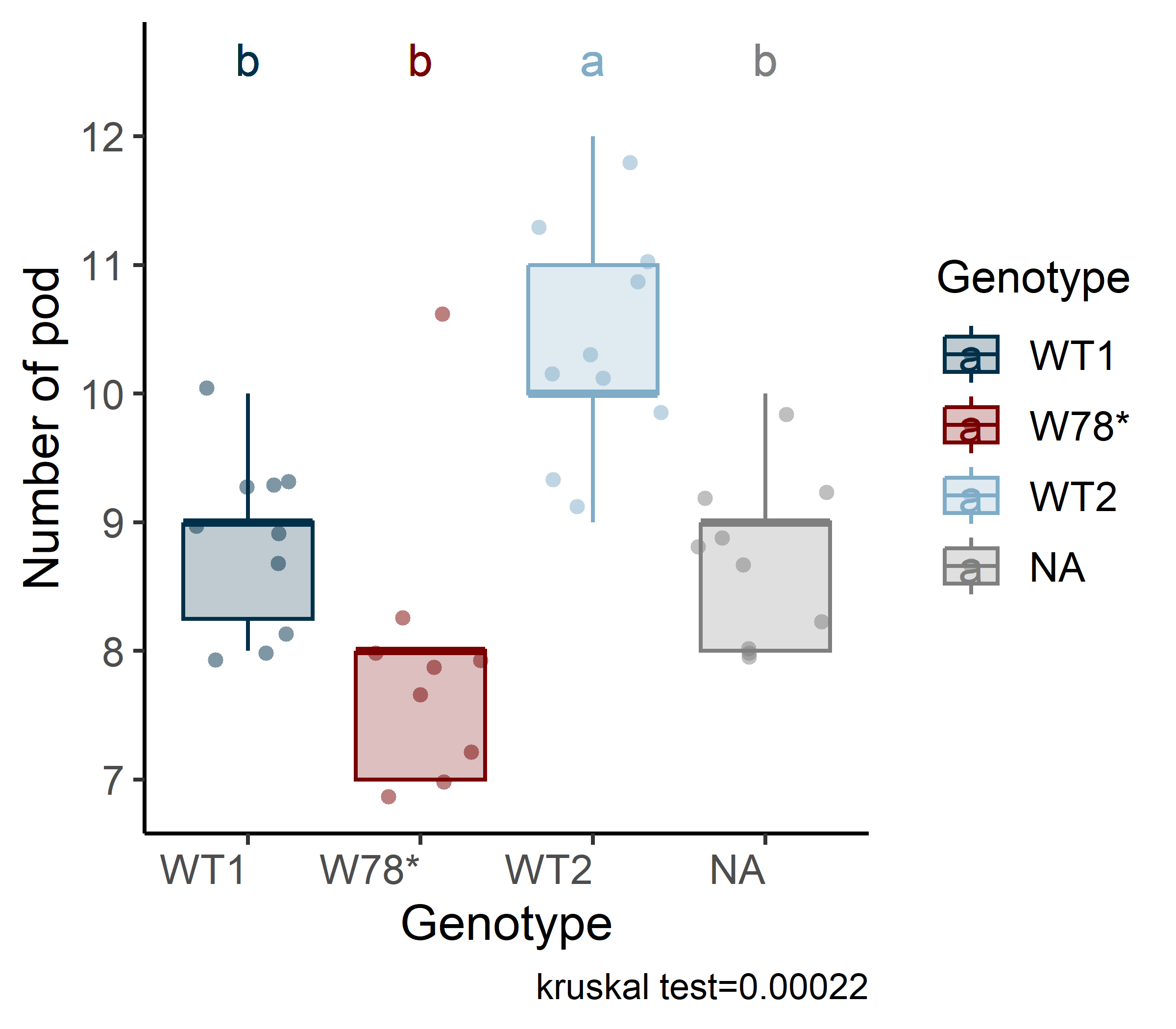
p <- stat_analyse(
    data=df_development %>% 
      as.data.frame(),
      #mutate(climat_condition=paste0(water_condition,"_",heat_condition)) %>% 
      #mutate(condition=factor(condition,levels=c("Sto_WW_OT","Stoc_WS_OT","Sto_WW_HS","Sto_WS_HS","Wen_WW_OT","Wen_WS_OT","Wen_WW_HS","Wen_WS_HS"))) %>% 
      
    column_value = "pod",
    category_variables = c("genotype"),
    grp_var = "",
    show_plot = T,
    outlier_show = F, 
    label_outlier = "plant_num",
    biologist_stats = T,
    Ylab_i =  "Number of pod",
    control_conditions = "",
    strip_normale = F,
    hex_pallet = c("#003049", "#780000", "#7FACC7", "#EC323E")
)

p <-p[["plot"]]+labs(color="Genotype",fill="Genotype",x="Genotype")
fig_export(here::here("report/physio/plot/development/development"), p, height_i = 3.5, width_i = 4, res_i = 600)