--- output: html_document editor_options: chunk_output_type: console --- ## Leaf chlorophyll content {#chlorophyll} ```{r} #pkg library (readxl)library (tidyverse)library (ggnewscale) # to have two scale_fill library (ggh4x)library (patchwork)#src source (here:: here ("src/function/stat_function/stat_analysis_main.R" )) # for make plot source (here:: here ("src/function/fig_export.R" )) # This function saves a given plot (plot_x) as both a PDF and a high-resolution PNG file at specified dimensions. #cosmetics = read_excel (here:: here ("data/color_palette.xlsm" )) %>% filter (set == "sulfure_condition" ) %>% :: select (color, treatment) %>% pull (color) %>% setNames (read_excel (here:: here ("data/color_palette.xlsm" )) %>% filter (set == "sulfure_condition" ) %>% pull (treatment)= read_excel (here:: here ("data/color_palette.xlsm" )) %>% filter (set == "mutant" ) %>% :: select (color, treatment) %>% pull (color) %>% setNames (read_excel (here:: here ("data/color_palette.xlsm" )) %>% filter (set == "mutant" ) %>% pull (treatment)``` [ experiment 2 ](#experimental_design) on 2 leaflets of leaves of both nodes 4 and 5; 2 to 4 leaflets of leaves of node 7; and 3 to 4 leaflets of leaves of node 9 or 10, on 4 to 6 plants per genotype and condition, at 11 to 12 time points. Height and number of nodes were measured on 6 plants for each genotype and condition at 3 time points, corresponding to the stage of leaf samplings (7, 29, and 37 DAP).```{r, eval = F} # Data importation df_spad_2021 = read.table(here::here("data/physio/SPAD_Serre_24_raw_data.txt"), dec = ",", sep = "\t", header = TRUE, as.is = FALSE) %>% dplyr::select(-c(Condition_Genotype, Replicate)) %>% dplyr::rename(plant_num = Plant_nb, sulfur_condition = Condition, genotype= Genotype, DAP = DAF) %>% mutate( genotype = case_when( genotype =="2684_WT" ~ "WT1", genotype =="2684_Homo" ~ "W78*", genotype =="4693_WT" ~ "WT2", genotype =="4693_Homo" ~ "E568K", ), sulfur_condition = ifelse(sulfur_condition =="S+", "SS", "SD"), type_genotype = ifelse(genotype %in% c("WT1", "WT2"), "WT", "Mut"), depodding = "All pod", sulfur_year_depodding = paste0(sulfur_condition, "_2021_", depodding), for_article = paste0(sulfur_condition, " - ", depodding) ) %>% pivot_longer(cols = c(N4_N5, N7, NR), names_to = "compartment", values_to = "spad") %>% mutate(sulfur_condition= fct_relevel(sulfur_condition, "SS", "SD"), genotype = fct_relevel(genotype, "WT1", "W78*", "WT2", "E568K"), compartment = fct_relevel(compartment, "NR", "N7","N4_N5"), type_genotype = fct_relevel(type_genotype, "WT", "Mut"), sulfur_year_depodding = fct_relevel(sulfur_year_depodding, "SS_2021_All pod", "SD_2021_All pod"), for_article = paste0(sulfur_condition, " - ", depodding) ) ############ Data importation SPAD DATA plant_info <- read_excel(here::here("data/plant_info.xlsx"), col_names = T) %>% dplyr::rename("position"= "tablar position") excel_sheets <- excel_sheets(here::here("data/physio/SPAD_greenhouse_2025_raw_data.xlsx"))[-1] # function to read one excel_sheet read_excel_spad <- function(sheet_name){ df_x <- read_excel(here::here("data/physio/SPAD_greenhouse_2025_raw_data.xlsx"), col_names = T, sheet = sheet_name) df_x_select <- df_x %>% dplyr::select(plant_num, date, N4_1, N4_2, N5_1, N5_2, N6_1, N6_2, N7_1, N7_2, NR_1, NR_2) %>% rowwise() %>% mutate(N4 = mean(c(N4_1, N4_2), na.rm = TRUE), N5 = mean(c(N5_1, N5_2), na.rm = TRUE), N4_N5 = mean (c(N4_1, N4_2, N5_1, N5_2), na.rm = TRUE), N6 = mean(c(N6_1, N6_2), na.rm = TRUE), N7 = mean(c(N7_1, N7_2), na.rm = TRUE), NR = mean(c(NR_1, NR_2), na.rm = TRUE)) %>% ungroup() %>% mutate(DAP = as.numeric(as.Date(date)-as.Date("2025-04-10")), sulfur_condition = "SD") %>% left_join(., read_excel(here::here("data/plant_info.xlsx"), col_names = T) %>% dplyr::rename("position"= "tablar position"), by = "plant_num") %>% mutate( depodding = ifelse(depodding %in% c("D", "FD"), "Consistent pod number", "All pod (2025)"), sulfur_year_depodding = paste0(sulfur_condition,"_2025_", depodding), for_article = paste0(sulfur_condition, " - ", depodding) ) %>% relocate(c(DAP, row,line, position, genotype, depodding, condition, sulfur_condition), .after = date) %>% filter(plant_num != 6) return(df_x_select) } #test = read_excel_spad(excel_sheets[1]) df_spad_2025_raw <- excel_sheets %>% lapply(read_excel_spad) %>% bind_rows() df_spad_2025 = df_spad_2025_raw %>% mutate(type_genotype = ifelse(genotype %in% c("WT1", "WT2"), "WT", "Mut") ) %>% dplyr::select(-c(N4_1, N4_2, N5_1, N5_2 , N6_1 , N6_2, N7_1 , N7_2, NR_1 ,NR_2)) %>% pivot_longer(cols = c(N4, N5,N4_N5 , N6, N7, NR), names_to = "compartment", values_to = "spad") %>% mutate(genotype = fct_relevel(genotype, "WT1", "W78*", "WT2", "E568K"), compartment = fct_relevel(compartment, "NR", "N7","N6", "N5", "N4"), type_genotype = fct_relevel(type_genotype, "WT", "Mut"), sulfur_year_depodding = fct_relevel(sulfur_year_depodding, "SD_2025_All pod (2025)", "SD_2025_Consistent pod number"), for_article = fct_relevel(for_article, "SD - All pod (2025)", "SD - Consistent pod number"), ) levels(as.factor(df_spad_2025$sulfur_year_depodding)) levels(as.factor(df_spad_2021$for_article)) levels(as.factor(df_spad_2025$date)) ``` # Visualisation ```{r, eval = F} p_spad_2021 = ggplot(df_spad_2021, aes(x = DAP, y = spad, color = genotype, fill = genotype, linetype = type_genotype)) + geom_point(alpha = 0.4, size = .7, shape = 16) + geom_smooth(se = T, linewidth = .8,alpha = .4) + facet_nested(compartment ~ sulfur_year_depodding, strip = strip_nested( background_x = list( element_rect(fill = sulfate_pallet[["SS"]]), element_rect(fill = sulfate_pallet[["SD"]]) ), background_y = list( element_rect(fill = "#EEF0D1"), element_rect(fill = "#C3D592"), element_rect(fill = "#97B953") ) )) + labs( x = "Days After Pollination (DAP)", y = "Chlorophyll content", color = "Genotype", fill = "Genotype", linetype = "Type of genotype" ) + theme_minimal() + theme( panel.grid.major = element_line(color = "gray85"), # Lignes de grille légères panel.grid.minor = element_blank(), # Suppression des petites grilles strip.text = element_text(face = "bold"), legend.position = "right" )+ scale_fill_manual(values = mutant_palette)+ scale_color_manual(values = mutant_palette) fig_export(here::here("report/physio/plot/spad_2021"), p_spad_2021, height_i = 6, width_i = 10, res_i = 600) # For 2025 p_spad_2025 <- df_spad_2025 %>% ggplot(., aes(x = DAP, y = spad, color = genotype, fill = genotype, linetype = type_genotype)) + geom_point(alpha = 0.4, size = .7, shape = 16) + geom_smooth(se = T, linewidth = .8,alpha = .4) + facet_nested(compartment ~ sulfur_year_depodding, strip = strip_nested( background_x = list( element_rect(fill = sulfate_pallet[["SD"]]) ), background_y = list( element_rect(fill = "#EEF0D1"), element_rect(fill = "#C3D592"), element_rect(fill = "#97B953"), element_rect(fill = "#789442"), element_rect(fill = "#4b5c29") ) )) + labs( x = "Days After Pollination (DAP)", y = "Chlorophyll content", color = "Genotype", fill = "Genotype", linetype = "Type of genotype" ) + theme_minimal() + theme( panel.grid.major = element_line(color = "gray85"), # Lignes de grille légères panel.grid.minor = element_blank(), # Suppression des petites grilles strip.text = element_text(face = "bold"), legend.position = "right" )+ scale_fill_manual(values = mutant_palette)+ scale_color_manual(values = mutant_palette) fig_export(here::here("report/physio/plot/spad_2025"), p_spad_2025, height_i = 6, width_i = 10, res_i = 600) ### combine both experiment p_bind_spad <- bind_rows(df_spad_2021, df_spad_2025) %>% filter(compartment %in% c("NR", "N7", "N4_N5")) %>% mutate(genotype = fct_relevel(genotype, "WT1", "W78*", "WT2", "E568K"), compartment = fct_relevel(compartment, "NR", "N7","N4_N5"), type_genotype = fct_relevel(type_genotype, "WT", "Mut"), depodding = factor(depodding,levels = c("Control", "Pod removal")), sulfur_year_depodding = fct_relevel(sulfur_year_depodding, "SS_2021_All pod", "SD_2021_All pod", "SD_2025_All pod (2025)", "SD_2025_Consistent pod number"), for_article = fct_relevel(for_article, "SD - All pod", "SS - All pod", "SD - All pod (2025)", "SD - Consistent pod number") ) %>% ggplot(., aes(x = DAP, y = spad, color = genotype, fill = genotype, linetype = type_genotype)) + geom_point(alpha = 0.4, size = .7, shape = 16) + geom_smooth(se = T, linewidth = .8,alpha = .4) + facet_nested(compartment ~ sulfur_year_depodding, strip = strip_nested( background_x = list( element_rect(fill = sulfate_pallet[["SS"]]), element_rect(fill = sulfate_pallet[["SD"]]), element_rect(fill = sulfate_pallet[["SD"]]), element_rect(fill = sulfate_pallet[["SD"]]) ), background_y = list( element_rect(fill = "#EEF0D1"), element_rect(fill = "#C3D592"), element_rect(fill = "#97B953") ) )) + labs( x = "Days After Pollination (DAP)", y = "Chlorophyll content", color = "Genotype", fill = "Genotype", linetype = "Type of genotype" ) + theme_minimal() + theme( panel.grid.major = element_line(color = "gray85"), # Lignes de grille légères panel.grid.minor = element_blank(), # Suppression des petites grilles strip.text = element_text(face = "bold"), legend.position = "right" )+ scale_fill_manual(values = mutant_palette)+ scale_color_manual(values = mutant_palette) fig_export(here::here("report/physio/plot/spad_all"), p_bind_spad, height_i = 6, width_i = 12, res_i = 300) # figure for article p_bind_spad_article <- bind_rows(df_spad_2021, df_spad_2025) %>% filter(compartment %in% c("NR", "N7", "N4_N5")) %>% filter(for_article != "SD - All pod (2025)") %>% mutate(genotype = fct_relevel(genotype, "WT1", "W78*", "WT2", "E568K"), compartment = fct_relevel(compartment, "NR", "N7","N4_N5"), type_genotype = fct_relevel(type_genotype, "WT", "Mut"), depodding = factor(depodding,levels = c("Control", "Pod removal")), sulfur_year_depodding = fct_relevel(sulfur_year_depodding, "SS_2021_All pod", "SD_2021_All pod", "SD_2025_Consistent pod number"), for_article = fct_relevel(for_article, "SS - All pod", "SD - All pod", "SD - Consistent pod number") ) %>% ggplot(., aes(x = DAP, y = spad, color = genotype, fill = genotype, linetype = type_genotype)) + geom_point(alpha = 0.4, size = .7, shape = 16) + geom_smooth(se = T, linewidth = .8,alpha = .4) + facet_nested(compartment ~ for_article, strip = strip_nested( background_x = list( element_rect(fill = sulfate_pallet[["SS"]]), element_rect(fill = sulfate_pallet[["SD"]]), element_rect(fill = sulfate_pallet[["SD"]]), element_rect(fill = sulfate_pallet[["SD"]]) ), background_y = list( element_rect(fill = "#EEF0D1"), element_rect(fill = "#C3D592"), element_rect(fill = "#97B953") ) )) + labs( x = "Days After Pollination (DAP)", y = "Chlorophyll content", color = "Genotype", fill = "Genotype", linetype = "Type of genotype" ) + theme_minimal() + theme( panel.grid.major = element_line(color = "gray85"), # Lignes de grille légères panel.grid.minor = element_blank(), # Suppression des petites grilles strip.text = element_text(face = "bold"), legend.position = "top" )+ scale_fill_manual(values = mutant_palette)+ scale_color_manual(values = mutant_palette) fig_export(here::here("report/physio/plot/spad_article"), p_bind_spad_article, height_i = 6, width_i = 9, res_i = 300) # More simple graph ? # df.summary2 <- df_spad %>% # dplyr::group_by(DAF, genotype, compartment, sulfur_condition) %>% # dplyr::summarise( # sd = sd(spad, na.rm = T), # len = mean(spad, na.rm = T) # ) # # ggplot(df.summary2, aes(DAF, len)) + # geom_errorbar( # aes(ymin = len-sd, ymax = len+sd, color = genotype), # position = position_dodge(1.5) # )+ # geom_line(aes(color = genotype),position = position_dodge(1.5))+ # scale_color_manual(values = c("#023e8a", "#c9184a", "#48cae4", "#ff758f"))+ # facet_nested(compartment ~ sulfur_condition, # strip = strip_nested( # background_x = list( # element_rect(fill = sulfate_pallet[["SS"]]), # element_rect(fill = sulfate_pallet[["SD"]]) # ), # background_y = list( # element_rect(fill = "#EEF0D1"), # element_rect(fill = "#C3D592"), # element_rect(fill = "#97B953") # ) # )) + # labs( # x = "Days After Flowering (DAF)", # y = "SPAD value", # color = "Genotype" # ) + # theme_minimal() # Stats only on N4_N5 in SS for SPAD at 35 DAF df_select = df_spad_2021 %>% filter(sulfur_condition == "SS", compartment == "N4_N5", DAP == 35 ) %>% drop_na(spad) p1 <- stat_analyse( data=df_select %>% as.data.frame() %>% mutate(genotype=fct_relevel(genotype, "WT1", "W78*", "WT2", "E568K")), #mutate(climat_condition=paste0(water_condition,"_",heat_condition)) %>% #mutate(condition=factor(condition,levels=c("Sto_WW_OT","Stoc_WS_OT","Sto_WW_HS","Sto_WS_HS","Wen_WW_OT","Wen_WS_OT","Wen_WW_HS","Wen_WS_HS"))) %>% column_value = "spad", category_variables = c("genotype"), grp_var = "", show_plot = T, outlier_show = F, label_outlier = "plant_num", biologist_stats = T, Ylab_i = "Chlorophyll content for SS and \nall pod condition in N4_N5 at 35 DAP", control_conditions = "", strip_normale = F, hex_pallet = mutant_palette ) p1_ex <-p1[["plot"]]+labs(color="Genotype",fill="Genotype",x="Genotype") fig_export(here::here("report/physio/plot/spad_SS_N4_N5_35DAF"), p1_ex, height_i = 4, width_i = 3.8, res_i = 600) # Stats only on N4_N5 in SD for SPAD at 35 DAF df_select = df_spad_2021 %>% filter(sulfur_condition == "SD", compartment == "N4_N5", DAP == 35 ) %>% drop_na(spad) p2 <- stat_analyse( data=df_select %>% as.data.frame() %>% mutate(genotype=fct_relevel(genotype, "WT1", "W78*", "WT2", "E568K")), #mutate(climat_condition=paste0(water_condition,"_",heat_condition)) %>% #mutate(condition=factor(condition,levels=c("Sto_WW_OT","Stoc_WS_OT","Sto_WW_HS","Sto_WS_HS","Wen_WW_OT","Wen_WS_OT","Wen_WW_HS","Wen_WS_HS"))) %>% column_value = "spad", category_variables = c("genotype"), grp_var = "", show_plot = T, outlier_show = F, label_outlier = "plant_num", biologist_stats = T, Ylab_i = "Chlorophyll content for SD and \nall pod condition in N4_N5 at 35 DAP", control_conditions = "", strip_normale = F, hex_pallet = mutant_palette ) p2_ex <-p2[["plot"]]+labs(color="Genotype",fill="Genotype",x="Genotype") fig_export(here::here("report/physio/plot/spad_SD_N4_N5_35DAF"), p2_ex, height_i = 4, width_i = 3.8, res_i = 600) # Stats only on N4_N5 in SD for SPAD at 35 DAF df_select = df_spad_2025 %>% filter(sulfur_condition == "SD", compartment == "N4_N5", DAP == 40, depodding == "Consistent pod number" ) %>% drop_na(spad) p3 <- stat_analyse( data=df_select %>% as.data.frame() %>% mutate(genotype=fct_relevel(genotype, "WT1", "W78*", "WT2", "E568K")), #mutate(climat_condition=paste0(water_condition,"_",heat_condition)) %>% #mutate(condition=factor(condition,levels=c("Sto_WW_OT","Stoc_WS_OT","Sto_WW_HS","Sto_WS_HS","Wen_WW_OT","Wen_WS_OT","Wen_WW_HS","Wen_WS_HS"))) %>% column_value = "spad", category_variables = c("genotype"), grp_var = "", show_plot = T, outlier_show = F, label_outlier = "plant_num", biologist_stats = T, Ylab_i = "Chlorophyll content for SD and consistent pod \n number condition in N4_N5 at 40 DAP", control_conditions = "", strip_normale = F, hex_pallet = mutant_palette ) p3_ex <-p3[["plot"]]+labs(color="Genotype",fill="Genotype",x="Genotype") fig_export(here::here("report/physio/plot/spad_SD_N4_N5_40DAF_consistent_number_pod"), p3_ex, height_i = 4, width_i = 3.8, res_i = 600) # for article pa = p1[["plot"]]+labs(color="Genotype",fill="Genotype",x="Genotype")+theme(legend.position = "none") pb = p2[["plot"]]+labs(color="Genotype",fill="Genotype",x="Genotype")+theme(legend.position = "none") pc = p3[["plot"]]+labs(color="Genotype",fill="Genotype",x="Genotype")+theme(legend.position = "none") p_combine <- (pa | pb | pc) fig_x <- (p_bind_spad_article / p_combine ) + plot_layout(heights = c(1.5, 1)) fig_export(here::here("report/physio/plot/spad_fig_article_x"), fig_x, height_i = 9, width_i = 10, res_i = 600) ``` 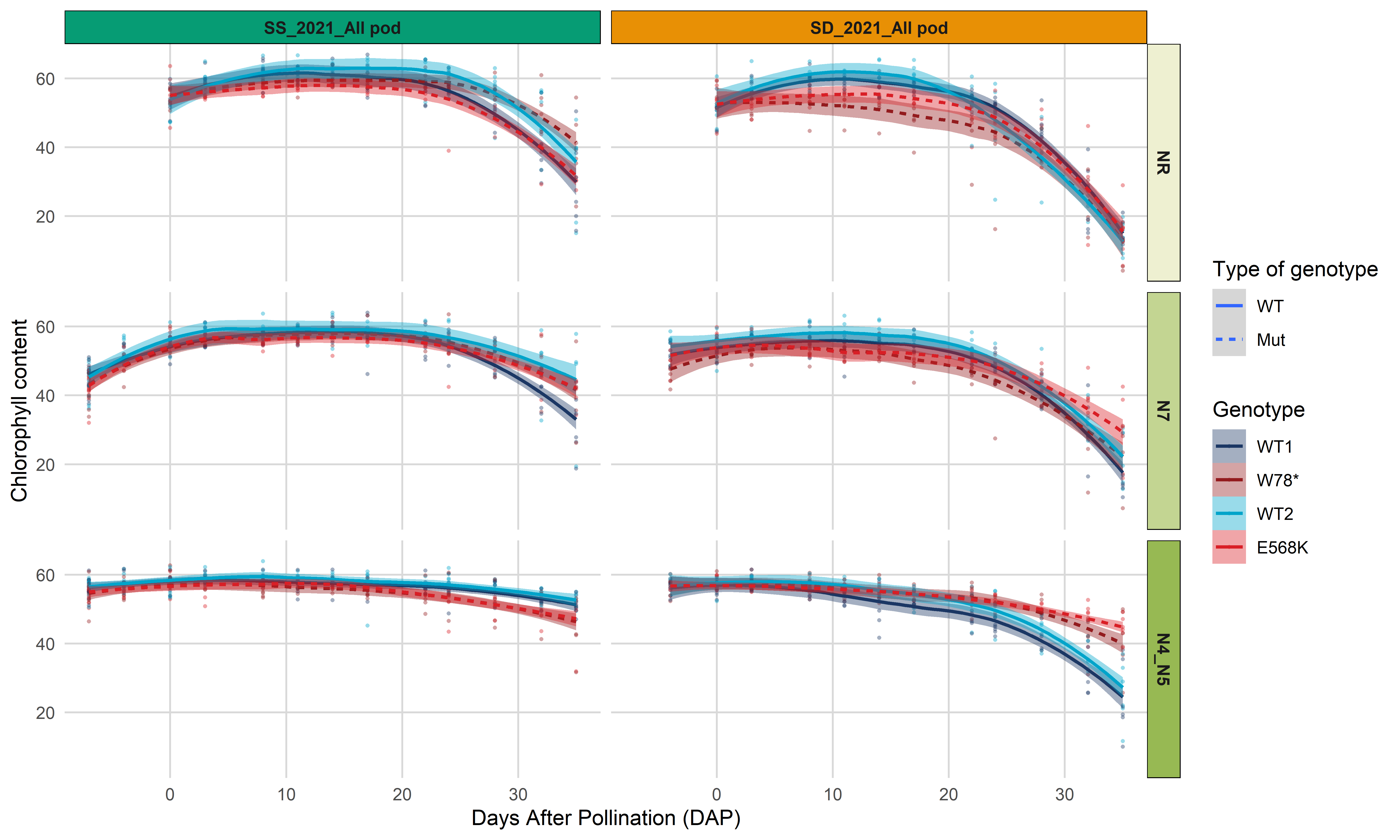  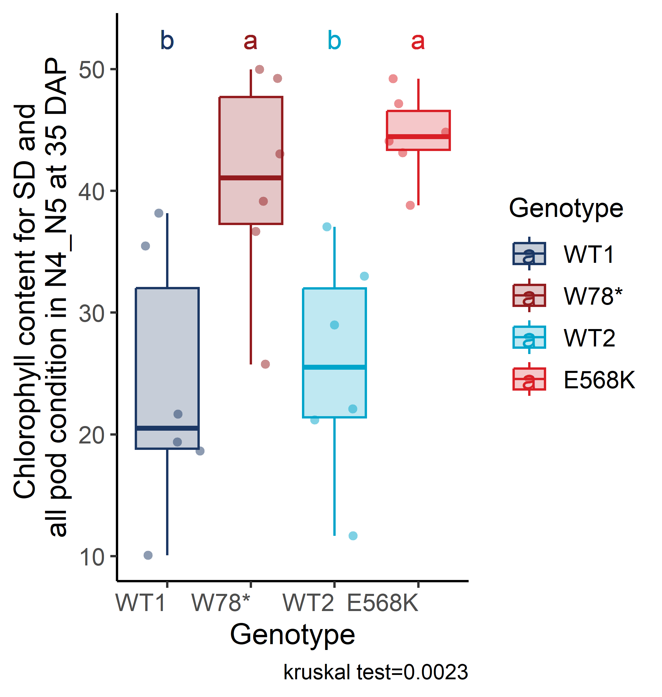 {width=300}

