#pkglibrary(tidyverse)library(here)library(readxl)library(ggnewscale) # to have two scale_filllibrary(ggh4x)library(ggstats)library(patchwork)# srcsource(here::here("src/function/stat_function/stat_analysis_main.R")) # for make plot source(here::here("src/function/fig_export.R")) # This function saves a given plot (plot_x) as both a PDF and a high-resolution PNG file at specified dimensions.# cosmeticssulfate_pallet=read_excel(here::here("data/color_palette.xlsm")) %>%filter(set =="sulfure_condition") %>% dplyr::select(color, treatment) %>%pull(color) %>%setNames(read_excel(here::here("data/color_palette.xlsm")) %>%filter(set =="sulfure_condition") %>%pull(treatment) )mutant_palette=read_excel(here::here("data/color_palette.xlsm")) %>%filter(set =="mutant") %>% dplyr::select(color, treatment) %>%pull(color) %>%setNames(read_excel(here::here("data/color_palette.xlsm")) %>%filter(set =="mutant") %>%pull(treatment) )
4.1 Data importation
There are 40 plants and two measurements are taken per plant. The first measurement is taken on the first leaflet of the fully developed leaf of the uppermost node, and the second on the first leaflet of the node below. The third measurement is taken on the first leaflet of the most developed leaf at the bottom of the plant.
name_files <-list.files(path =here("data/physio/LI-COR_LI-600"),pattern ="\\.csv$", full.names =TRUE)df_licor <-map_dfr(name_files, ~read_csv(.x, skip =1, col_names =TRUE, show_col_types =FALSE) %>%mutate(source_file =basename(.x), # Nom du fichier sans le cheminleaf_num =str_extract(source_file, "(?<=leaf_)\\d+") %>%as.integer() # extrait le numéro après "leaf_" )) %>%drop_na(configName) %>%select(-any_of(c("configAuthor", "configName", "remark", "...8", "...9"))) %>%rename(obs ="Obs#") %>%mutate(Time =hms(Time) +hours(7),Time =format(Time, "%H:%M:%S"),record =as.numeric(Record) ) %>%select(-Record) %>%mutate(across(where(~is.character(.) &&all(!is.na(suppressWarnings(as.numeric(.))))),~as.numeric(.)))# Add the number of the leaf where a measure has been carried out and the plant_informationplant_info <-read_excel(here::here("data/plant_info.xlsx"), col_names = T) %>% dplyr::rename("position"="tablar position")n_files <-length(name_files)df_licor <- df_licor %>%mutate(plant_num =rep(1:40, times = n_files)) %>%#mutate(plant_num = record) %>% left_join(plant_info, by ="plant_num") %>%mutate(genotype=fct_relevel(genotype, "WT1", "W78*", "WT2", "E568K")) %>%filter(plant_num!=6) %>%mutate(DAP =as.numeric(as.Date(Date)-as.Date("2025-04-10")), leaf_stage =case_when( leaf_num ==1~"Last fully expanded leaf", # première feuille complètement ouverte leaf_num ==2~"First reproductive node", # premier nœud reproducteur leaf_num ==3~"Fourth vegetative node"# quatrième nœud végétatif ),leaf_stage =factor(leaf_stage,levels =c("Last fully expanded leaf","First reproductive node","Fourth vegetative node")) ) %>%mutate(depodding =ifelse(depodding %in%c("D", "FD"), "Pod removal", "Control"))# export resultswrite_csv(x = df_licor, file = here::here("data/physio/LI-COR_LI-600/output/raw_licor.csv"))
4.2 Quick observation of results
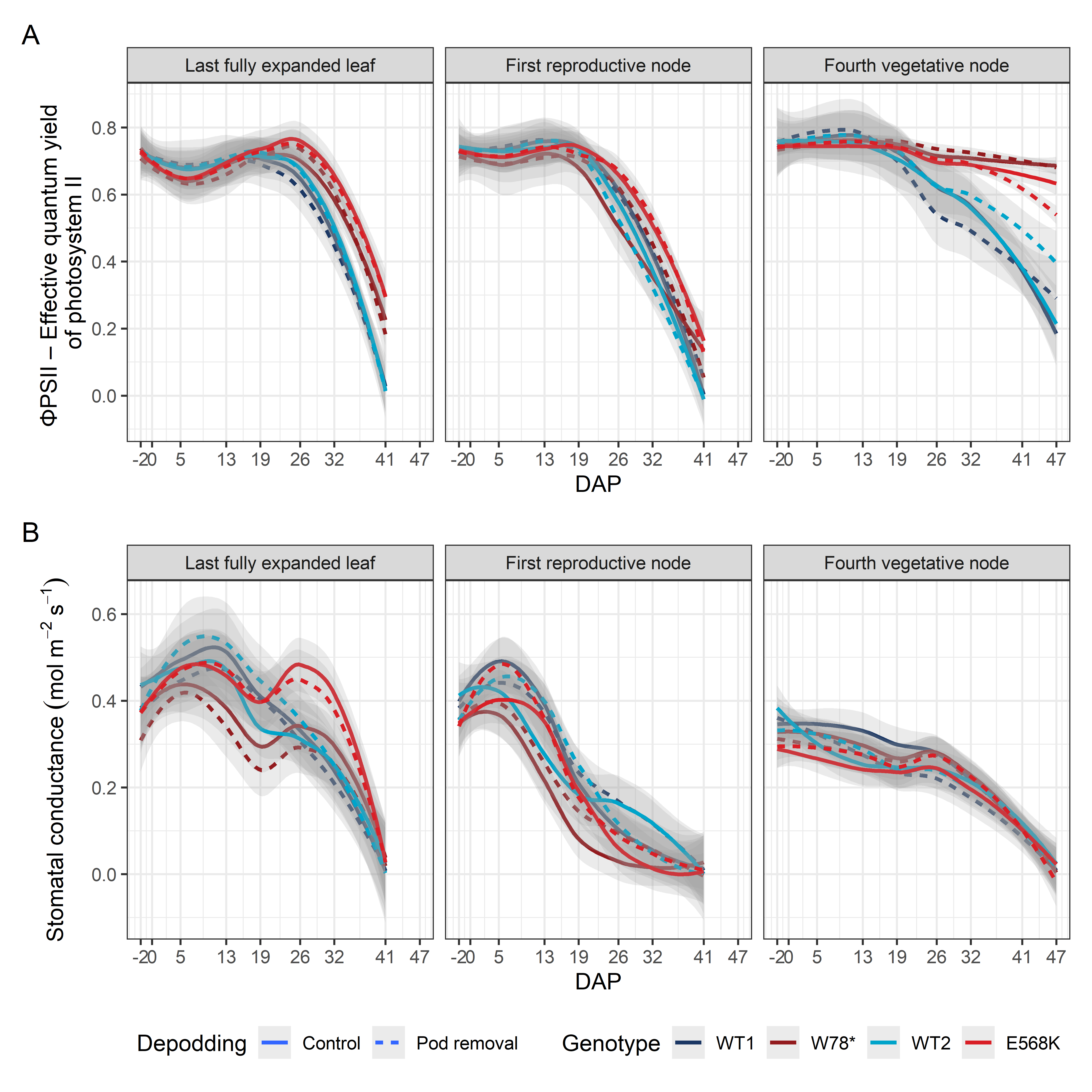
For stomatal conductance to water vapour, we look to see if there is an environmental effect.
Code
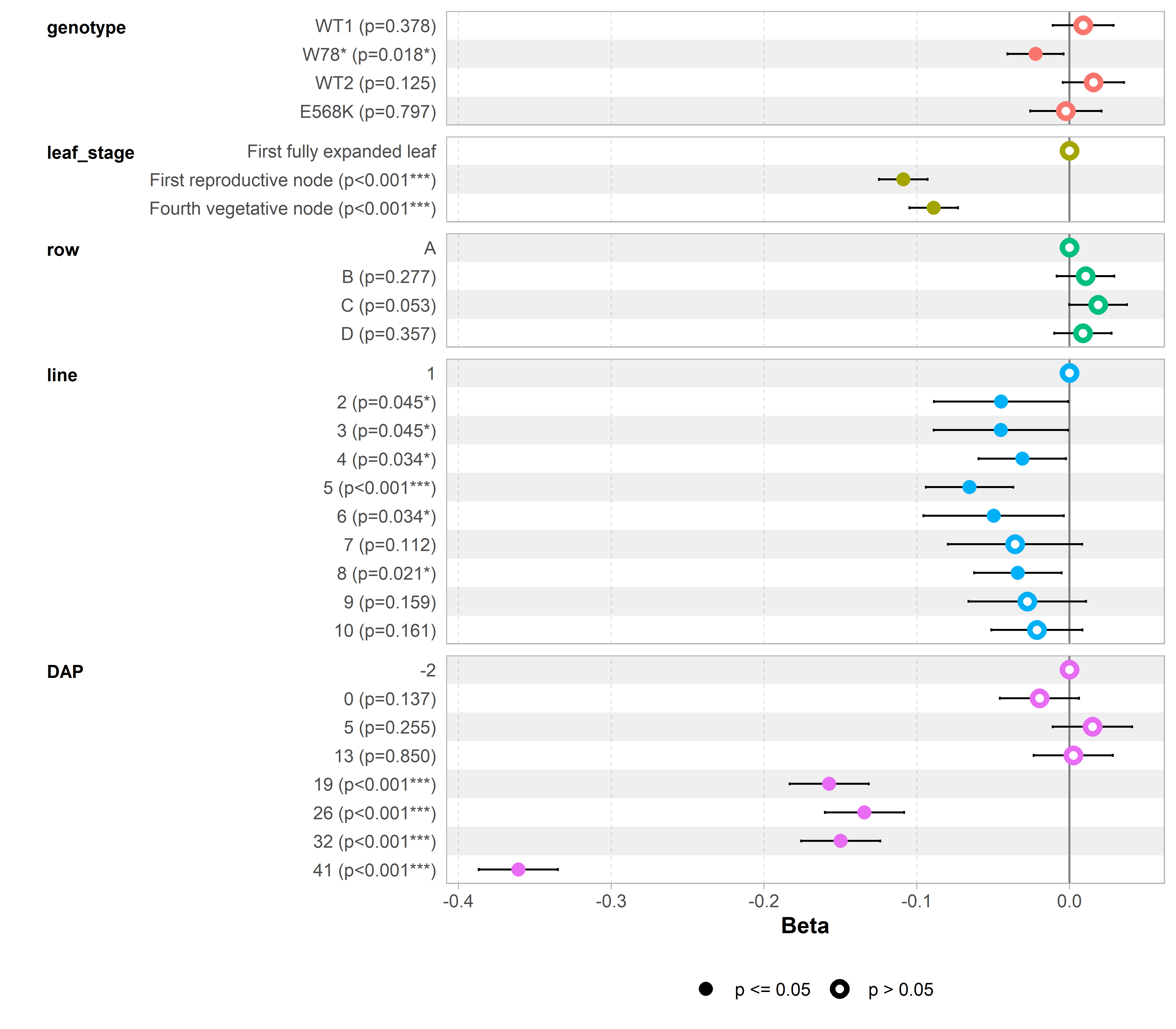
df_licor <-read_csv(here::here("data/physio/LI-COR_LI-600/output/raw_licor.csv"), show_col_types =FALSE) %>%mutate(depodding =as.factor(depodding),depodding =factor(depodding,levels =c("Control","Pod removal")))%>%mutate(plant_num =as.factor(plant_num),leaf_stage =as.factor(leaf_stage),leaf_stage =factor(leaf_stage,levels =c("Last fully expanded leaf","First reproductive node","Fourth vegetative node")),line =as.factor(line),genotype =as.factor(genotype),genotype=fct_relevel(genotype, "WT1", "W78*", "WT2", "E568K"), DAP =as.factor(DAP)) # %>% # mutate(DAP = relevel(DAP, ref = "0"))##### Linea mixed model ######contrasts(df_licor$genotype) <- contr.sum # to say look at the big average only for genotype (juste an other representation)mod1=lm(formula = gsw ~ genotype+leaf_stage+row+line+DAP+ depodding, data = df_licor)p_x<-ggcoef_model(mod1)fig_export(here::here("report/physio/plot/licor/ggcoef_model_gsw"), p_x, height_i =7, width_i =8, res_i =600)
There is a strong effect of the genotype (whether it’s a mutant or not), a strong effect of the leaf being analyzed and a strong effect of the position in the greenhouse, particularly the row. There is no line effect. So i need to correction for spatial trends.
4.3 Correction for spatial trends
The first step when modeling platform experiment data with the statgenHTP package is creating an object of class TP (Time Points). In this object, the time points are split into single data.frames. It is then used throughout the statgenHTP package as input for analyses.
4.4 Analysis of corrected results
Code
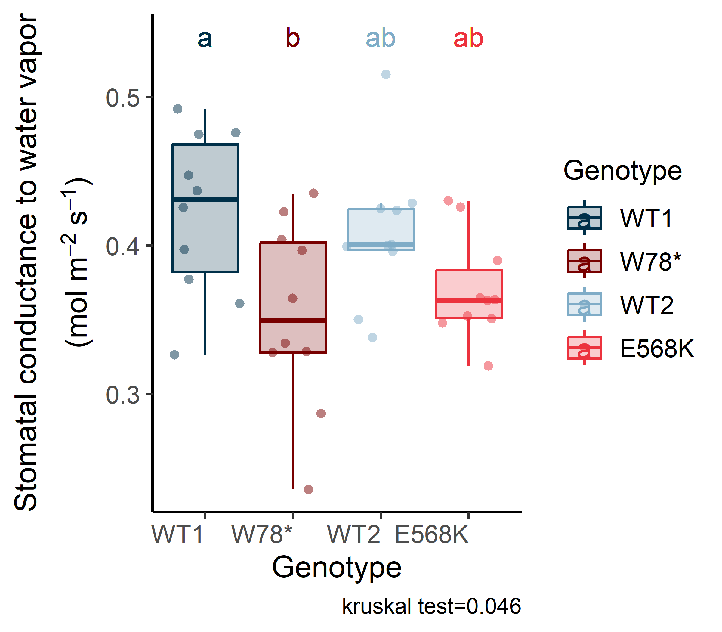
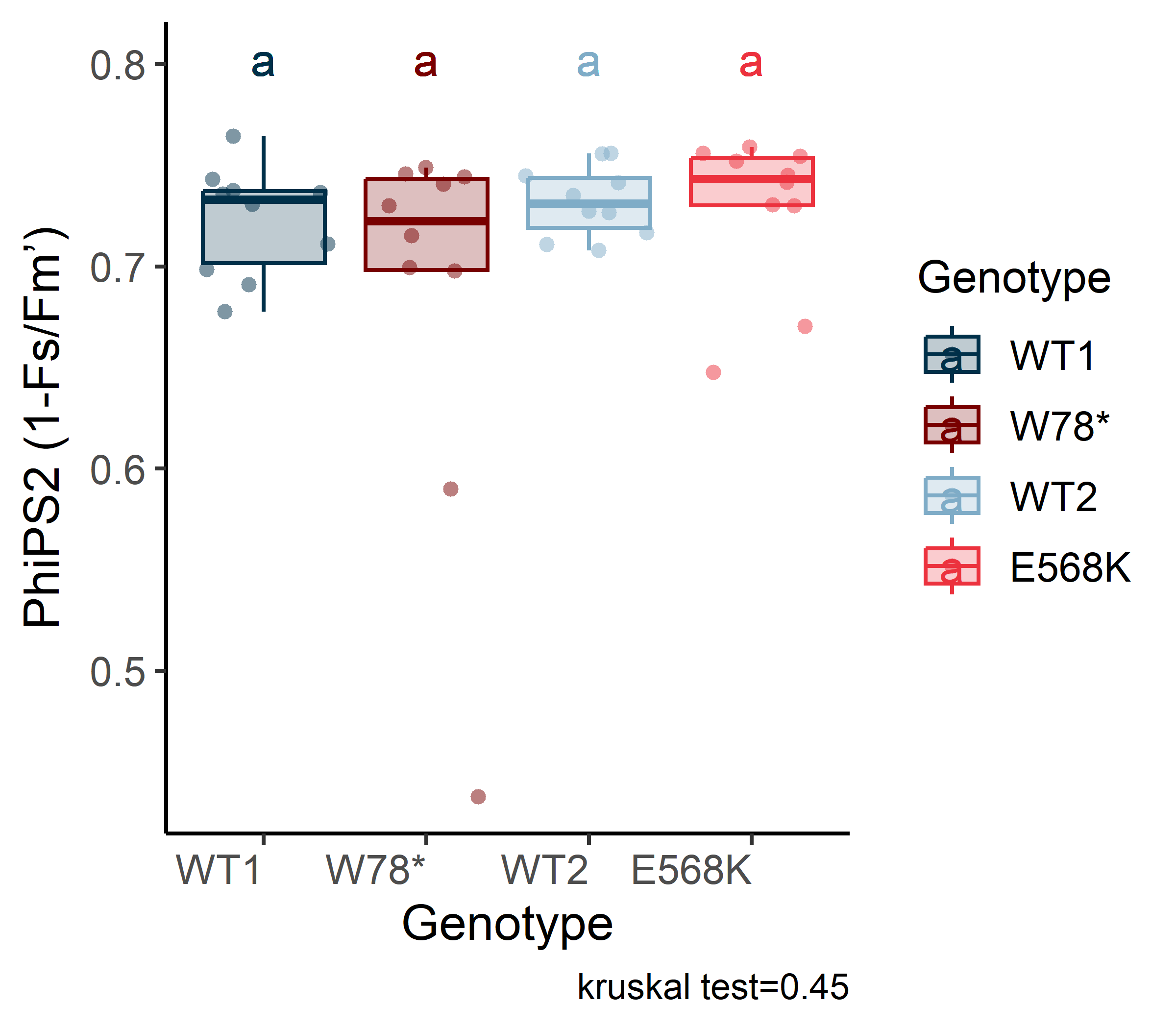
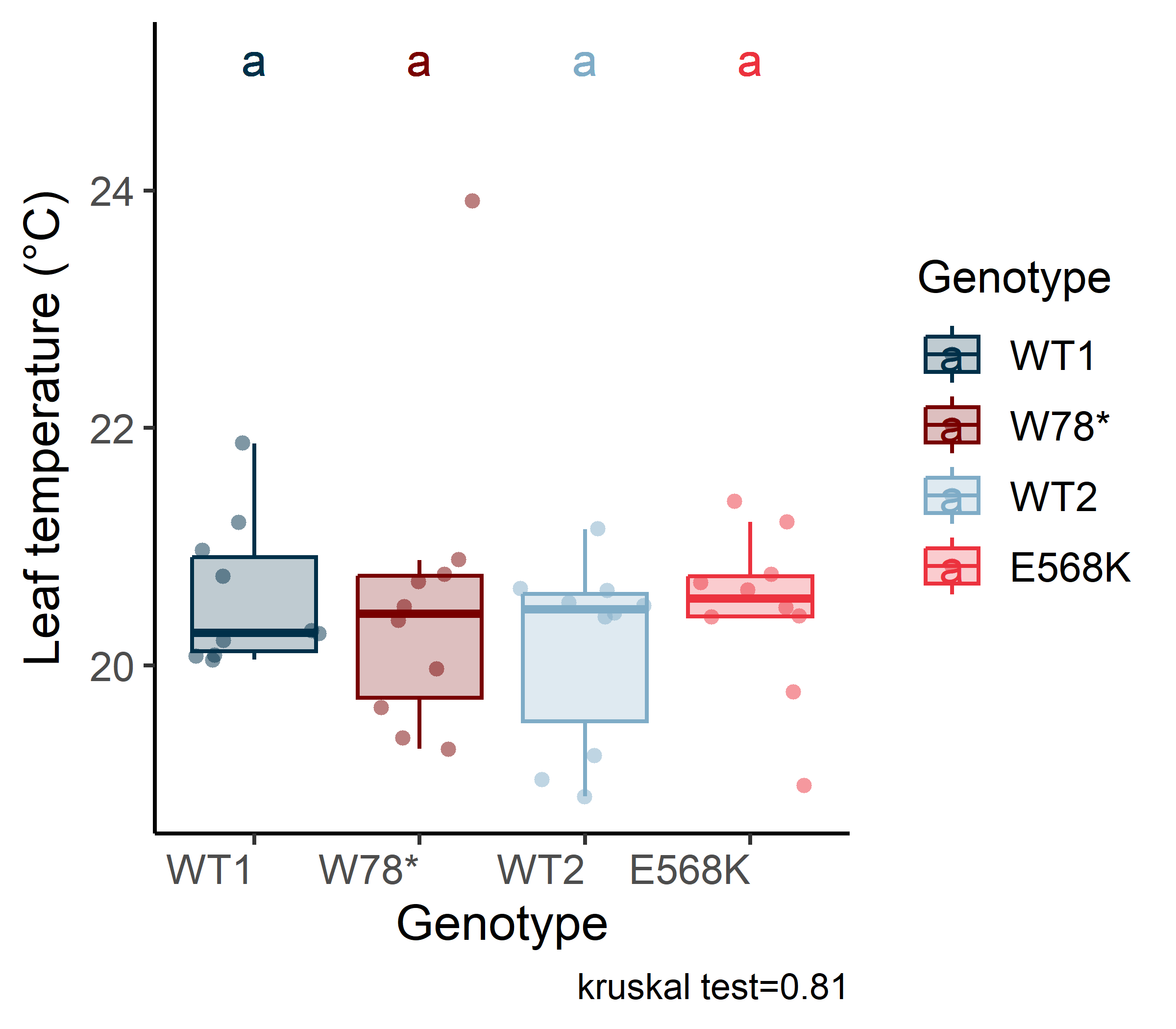
df_licor_leaf_1 = df_licor %>%filter(leaf_num ==1)df_licor_leaf_2 = df_licor %>%filter(leaf_num ==2)df_licor_leaf_3 = df_licor %>%filter(leaf_num ==3)df_licor_leaf_mean = df_licor %>% dplyr::group_by(plant_num, genotype) %>% dplyr::summarise(gsw=mean(gsw), PhiPS2=mean(PhiPS2), Tleaf=mean(Tleaf))# gswp <-stat_analyse(data=df_licor_leaf_2 %>%as.data.frame() %>%mutate(genotype=fct_relevel(genotype, "WT1", "W78*", "WT2", "E568K")),#mutate(climat_condition=paste0(water_condition,"_",heat_condition)) %>% #mutate(condition=factor(condition,levels=c("Sto_WW_OT","Stoc_WS_OT","Sto_WW_HS","Sto_WS_HS","Wen_WW_OT","Wen_WS_OT","Wen_WW_HS","Wen_WS_HS"))) %>% column_value ="gsw",category_variables =c("genotype"),grp_var ="",show_plot = T,outlier_show = F, label_outlier ="plant_num",biologist_stats = T,Ylab_i =expression(atop("Stomatal conductance to water vapor", "(mol m"^{-2}~"s"^{-1}*")")),control_conditions ="",strip_normale = F,hex_pallet =c("#003049", "#780000", "#7FACC7", "#EC323E"))p <-p[["plot"]]+labs(color="Genotype",fill="Genotype",x="Genotype")fig_export(here::here("report/physio/plot/licor/gsw_leaf_3"), p, height_i =3.5, width_i =4, res_i =600)##### Linea mixed model ######contrasts(df_licor$genotype) <- contr.sum # to say look at the big average only for genotype (juste an other representation)mod1=lm(formula = gsw ~ genotype+leaf_num+row+line, data = df_licor)p_x<-ggcoef_model(mod1)fig_export(here::here("report/physio/plot/licor/ggcoef_model_gsw.svg"), p_x, height_i =4, width_i =6, res_i =600)# Modèle avec uniquement la positionmod_position <-lm(gsw ~ row + line, data = df_licor)# Résidus = gsw "corrigé" de l'effet de la positiondf_licor <- df_licor %>%mutate(gsw_corrected =resid(mod_position))contrasts(df_licor$genotype) <- contr.sum # to say look at the big average only for genotype (juste an other representation)mod1_corr <-lm(gsw_corrected ~ genotype + leaf_num, data = df_licor)p_x <-ggcoef_model(mod1_corr)df_licor_leaf_2 = df_licor %>%filter(leaf_num ==3)p <-stat_analyse(data=df_licor_leaf_2 %>%as.data.frame() %>%mutate(genotype=fct_relevel(genotype, "WT1", "W78*", "WT2", "E568K")),#mutate(climat_condition=paste0(water_condition,"_",heat_condition)) %>% #mutate(condition=factor(condition,levels=c("Sto_WW_OT","Stoc_WS_OT","Sto_WW_HS","Sto_WS_HS","Wen_WW_OT","Wen_WS_OT","Wen_WW_HS","Wen_WS_HS"))) %>% column_value ="gsw_corrected",category_variables =c("genotype"),grp_var ="",show_plot = T,outlier_show = F, label_outlier ="plant_num",biologist_stats = T,Ylab_i =expression(atop("Stomatal conductance to water vapor", "(mol m"^{-2}~"s"^{-1}*")")),control_conditions ="",strip_normale = F,hex_pallet =c("#003049", "#780000", "#7FACC7", "#EC323E"))p <-p[["plot"]]+labs(color="Genotype",fill="Genotype",x="Genotype")fig_export(here::here("report/physio/plot/licor/gsw_leaf_2_corrected"), p, height_i =3.5, width_i =4, res_i =600)# fluorop <-stat_analyse(data=df_licor_leaf_3 %>%as.data.frame() %>%mutate(genotype=fct_relevel(genotype, "WT1", "W78*", "WT2", "E568K")),#mutate(climat_condition=paste0(water_condition,"_",heat_condition)) %>% #mutate(condition=factor(condition,levels=c("Sto_WW_OT","Stoc_WS_OT","Sto_WW_HS","Sto_WS_HS","Wen_WW_OT","Wen_WS_OT","Wen_WW_HS","Wen_WS_HS"))) %>% column_value ="PhiPS2",category_variables =c("genotype"),grp_var ="",show_plot = T,outlier_show = F, label_outlier ="plant_num",biologist_stats = T,Ylab_i =expression("PhiPS2 (1-Fs/Fm’)"),control_conditions ="",strip_normale = F,hex_pallet =c("#003049", "#780000", "#7FACC7", "#EC323E"))p <-p[["plot"]]+labs(color="Genotype",fill="Genotype",x="Genotype")fig_export(here::here("report/physio/plot/licor/PhiPS2_leaf_3"), p, height_i =3.5, width_i =4, res_i =600)# temperature leafp <-stat_analyse(data=df_licor_leaf_2 %>%as.data.frame() %>%mutate(genotype=fct_relevel(genotype, "WT1", "W78*", "WT2", "E568K")),#mutate(climat_condition=paste0(water_condition,"_",heat_condition)) %>% #mutate(condition=factor(condition,levels=c("Sto_WW_OT","Stoc_WS_OT","Sto_WW_HS","Sto_WS_HS","Wen_WW_OT","Wen_WS_OT","Wen_WW_HS","Wen_WS_HS"))) %>% column_value ="Tleaf",category_variables =c("genotype"),grp_var ="",show_plot = T,outlier_show = F, label_outlier ="plant_num",biologist_stats = T,Ylab_i =expression("Leaf temperature (°C)"),control_conditions ="",strip_normale = F,hex_pallet =c("#003049", "#780000", "#7FACC7", "#EC323E"))p <-p[["plot"]]+labs(color="Genotype",fill="Genotype",x="Genotype")fig_export(here::here("report/physio/plot/licor/Tleaf_leaf_2"), p, height_i =3.5, width_i =4, res_i =600)df_licor_leaf_choice <- df_licor_leaf_2 %>% dplyr::rename("Fm_bis"="Fm'")vars_non_nulles <- df_licor_leaf_choice %>% dplyr::select(-c("obs","plant_num","line","record")) %>% dplyr::select(where(is.numeric)) %>% dplyr::summarise(across(everything(), var, na.rm =TRUE)) %>%pivot_longer(everything(), names_to ="variable", values_to ="variance") %>%filter(variance !=0) %>%pull(variable)for (i in vars_non_nulles){ p <-stat_analyse(data=df_licor_leaf_choice %>%as.data.frame() %>%mutate(genotype=fct_relevel(genotype, "WT1", "W78*", "WT2", "E568K")),#mutate(climat_condition=paste0(water_condition,"_",heat_condition)) %>% #mutate(condition=factor(condition,levels=c("Sto_WW_OT","Stoc_WS_OT","Sto_WW_HS","Sto_WS_HS","Wen_WW_OT","Wen_WS_OT","Wen_WW_HS","Wen_WS_HS"))) %>% column_value = i,category_variables =c("genotype"),grp_var ="",show_plot = T,outlier_show = F, label_outlier ="plant_num",biologist_stats = T,Ylab_i = i,control_conditions ="",strip_normale = F,hex_pallet =c("#003049", "#780000", "#7FACC7", "#EC323E"))p <-p[["plot"]]+labs(color="Genotype",fill="Genotype",x="Genotype")fig_export(here::here(paste0("report/physio/plot/licor/test/",i)), p, height_i =3.5, width_i =4, res_i =600, format ="png")}