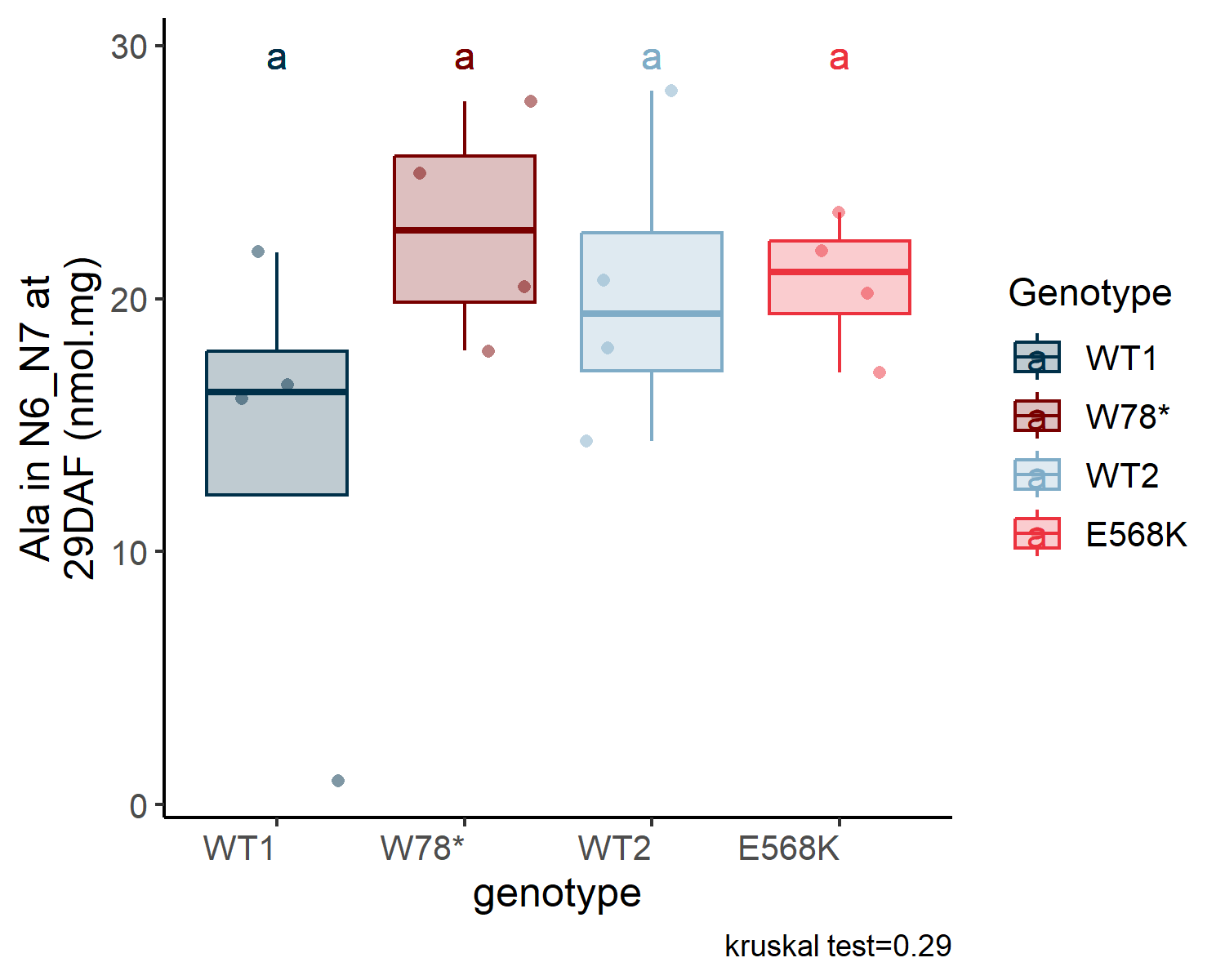
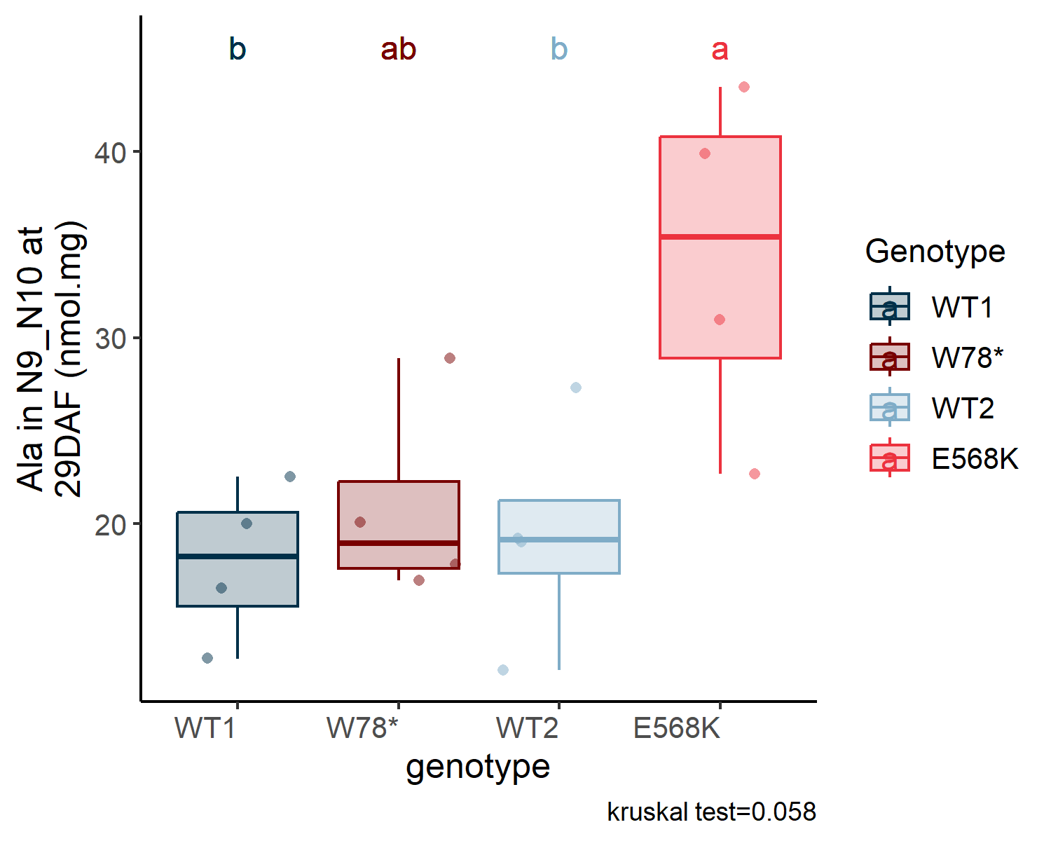
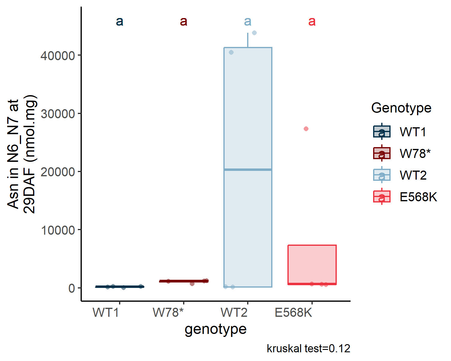
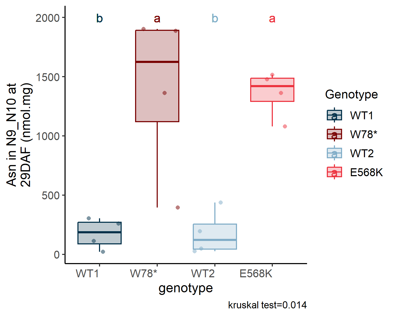
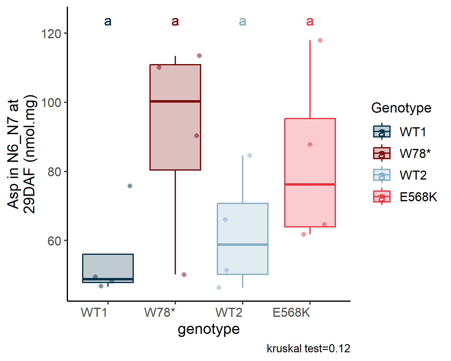
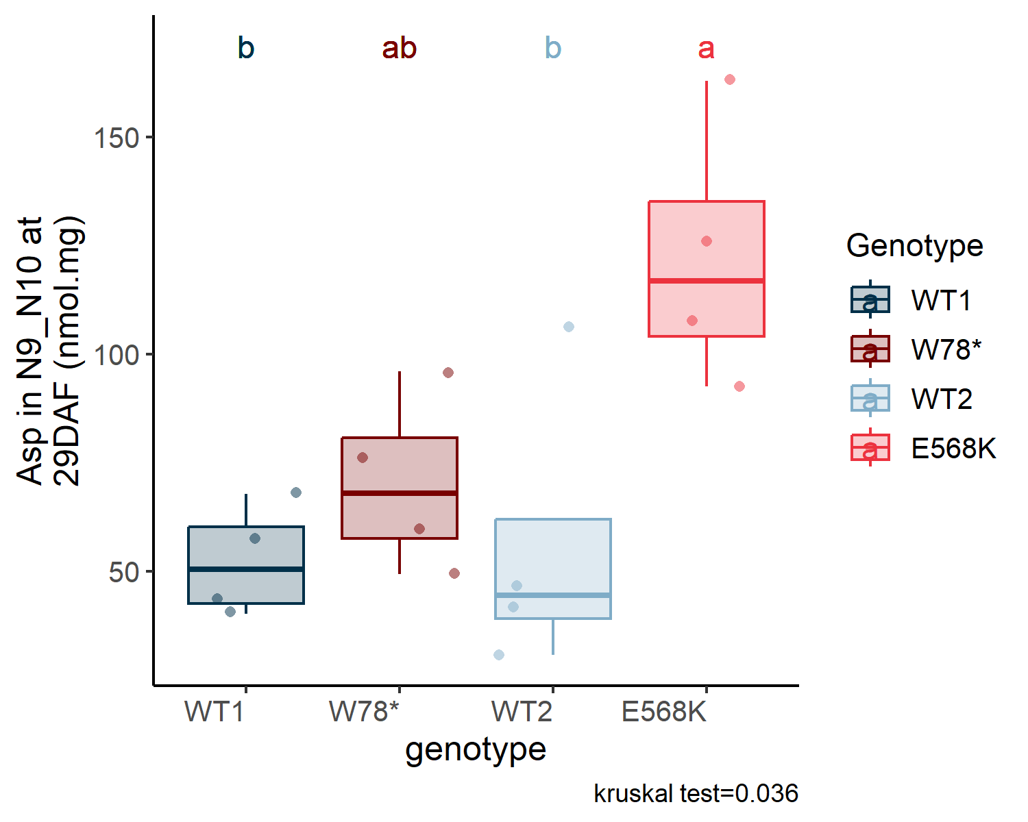
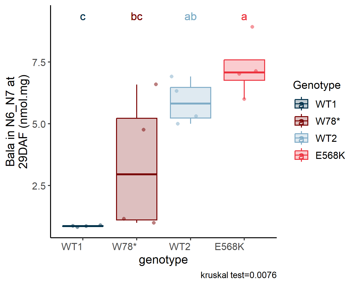
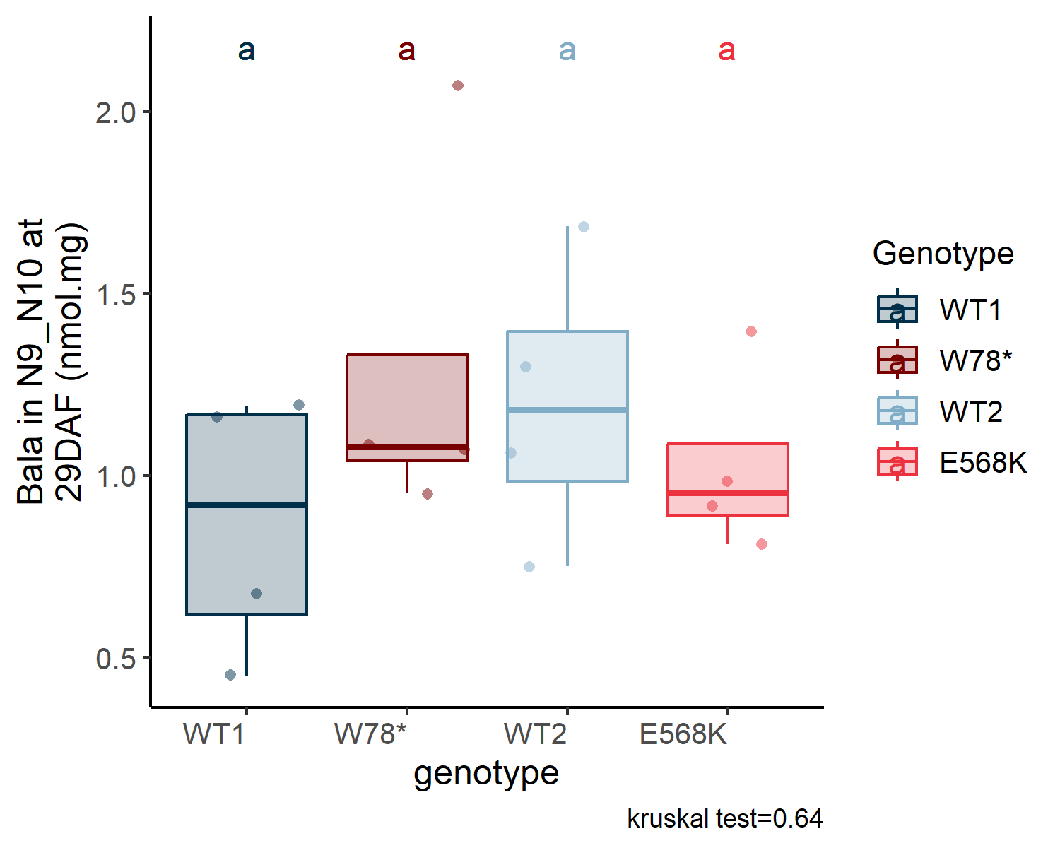
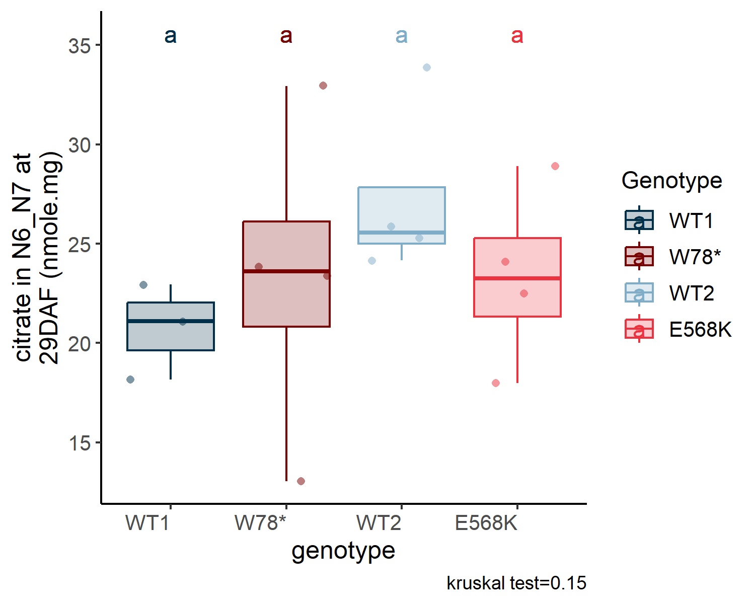
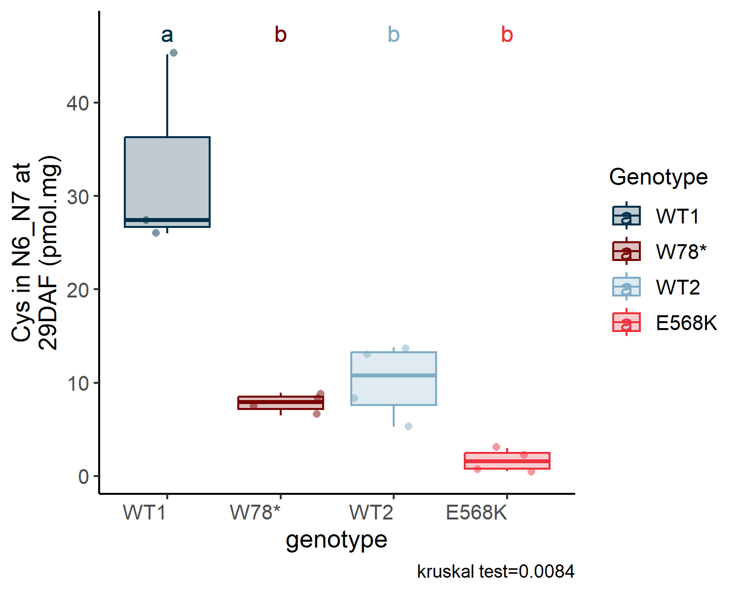
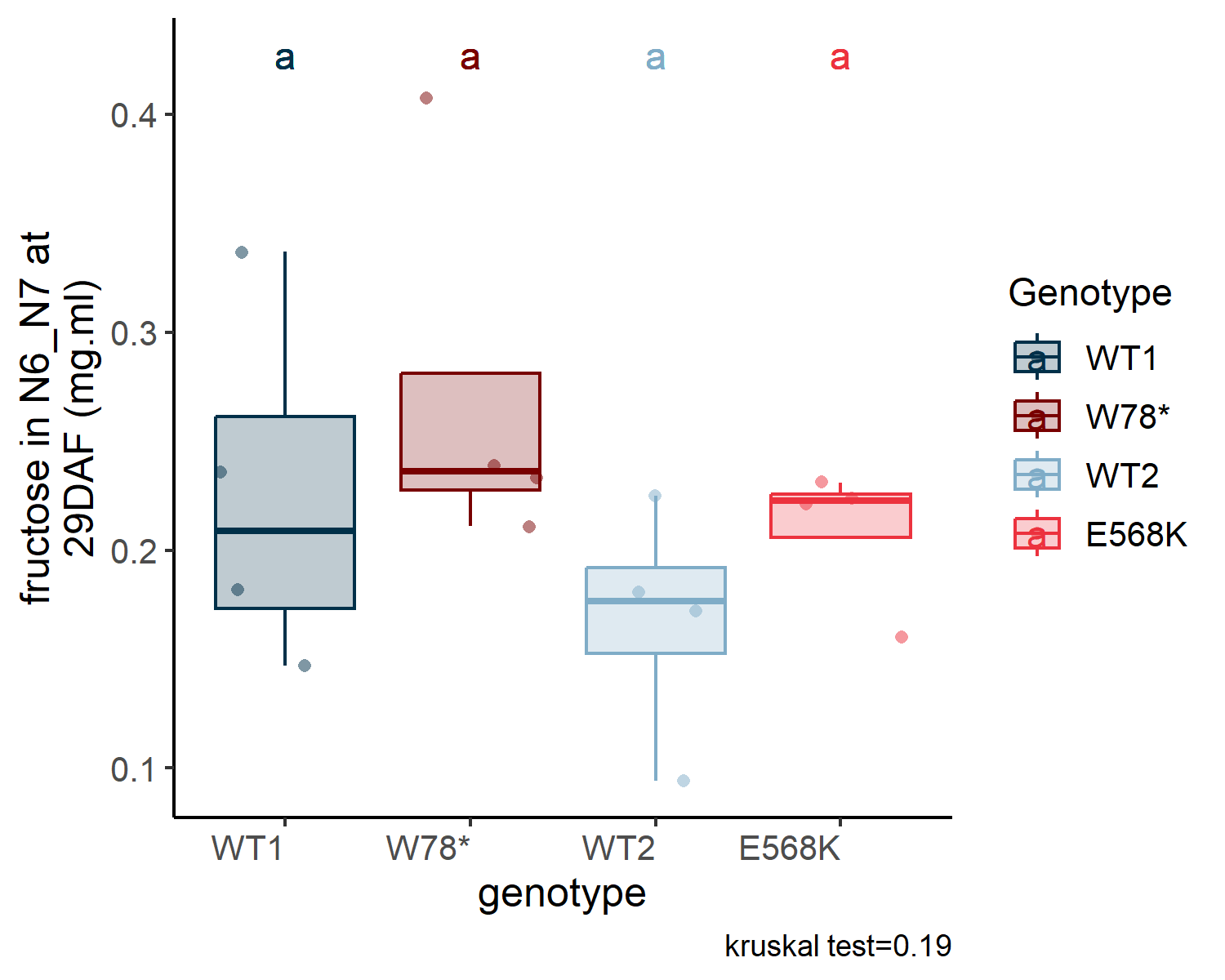
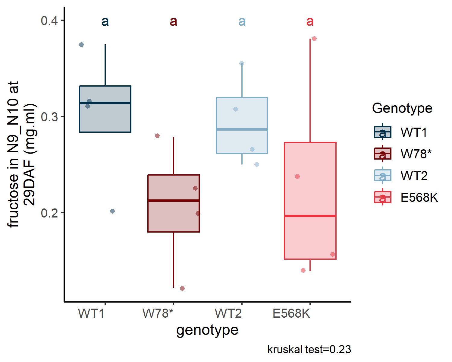
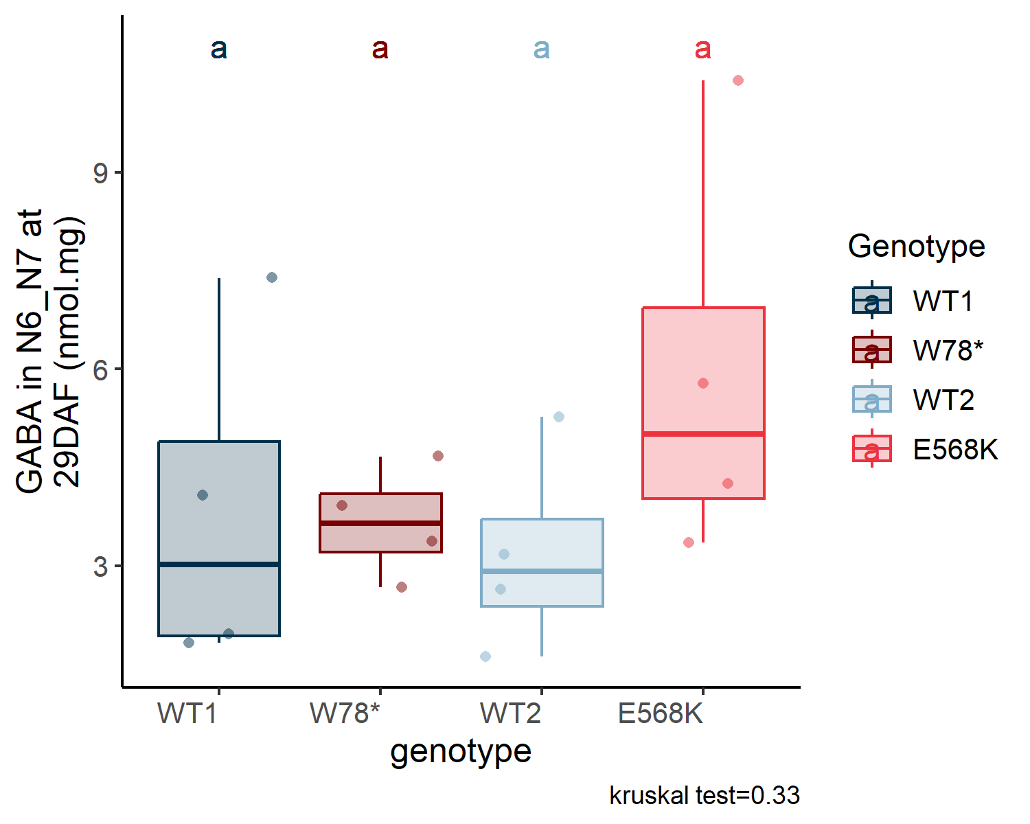
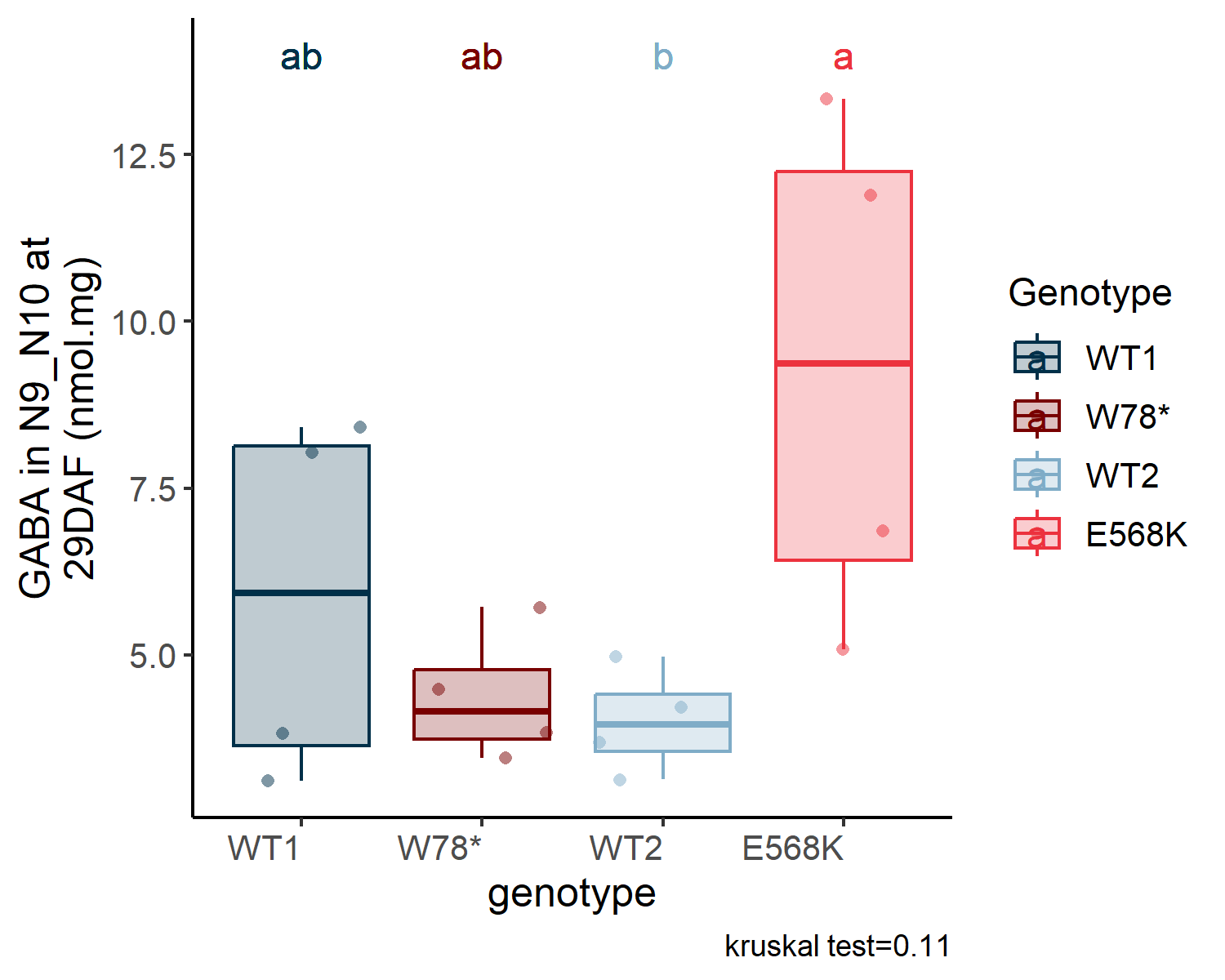
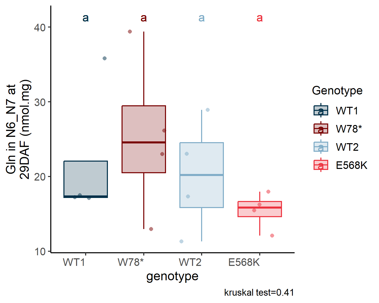
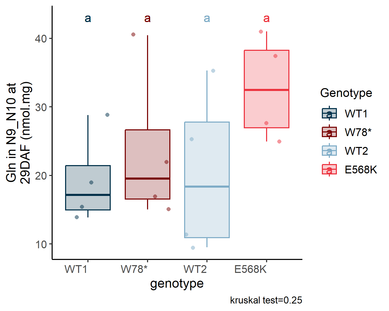
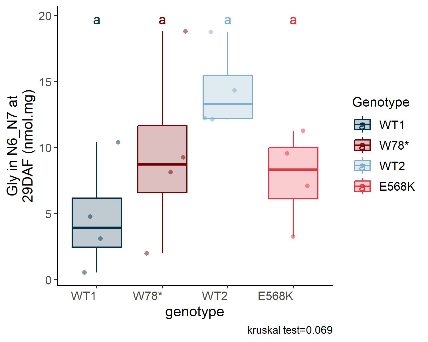
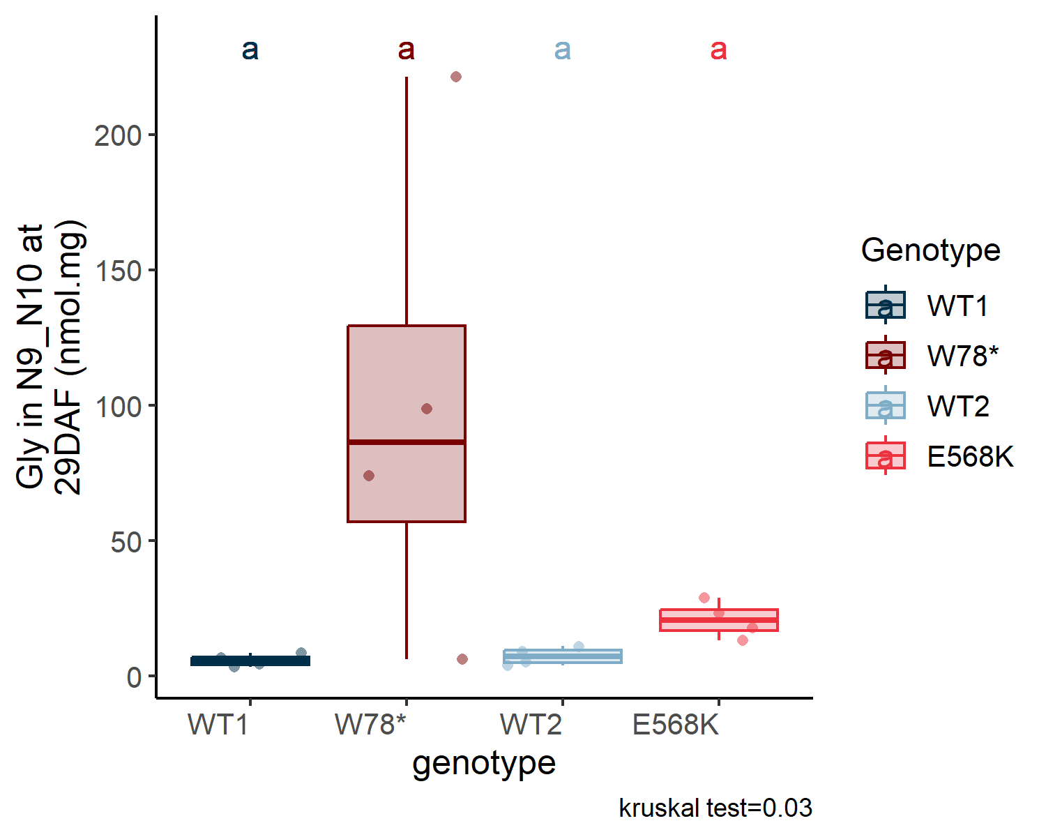
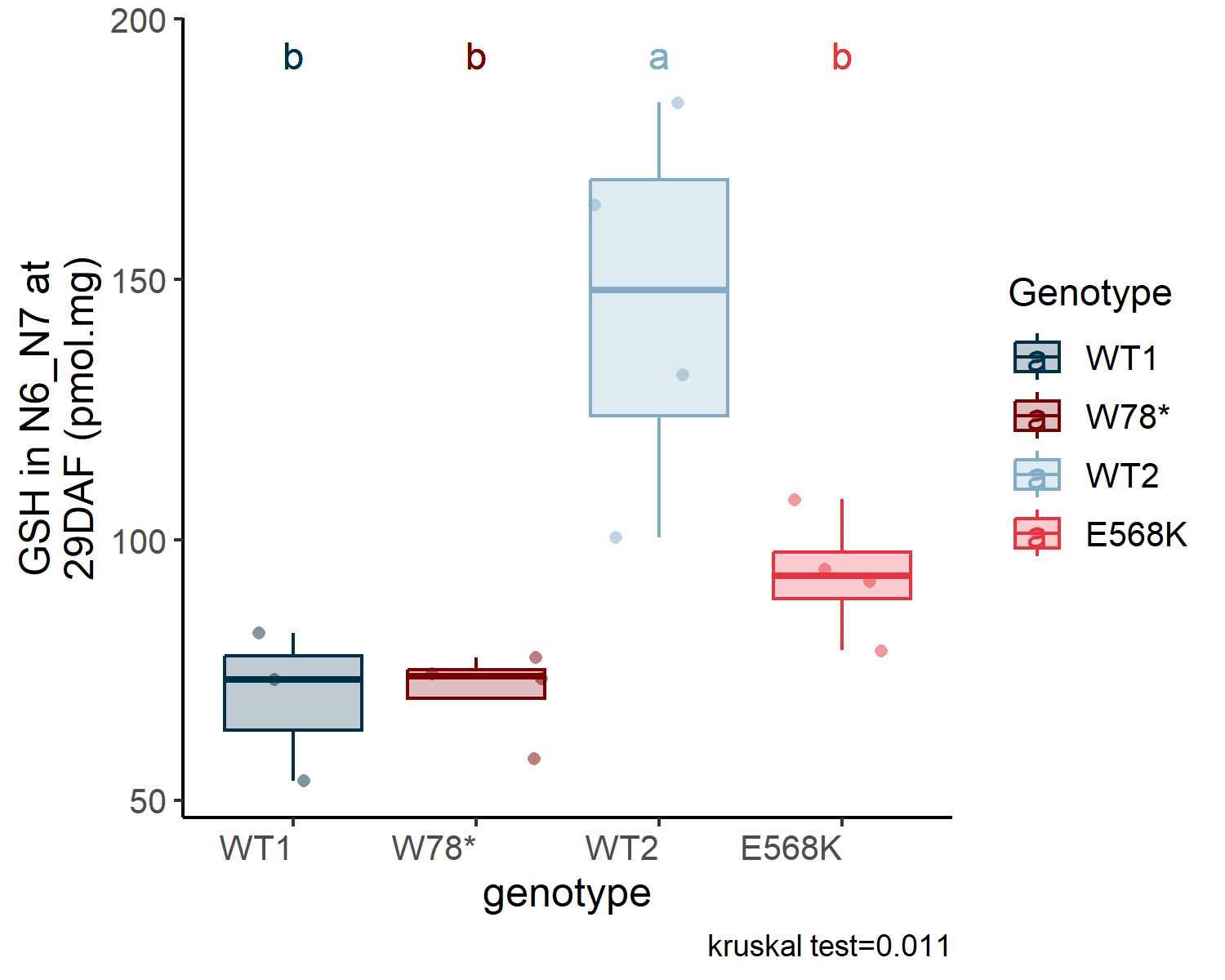
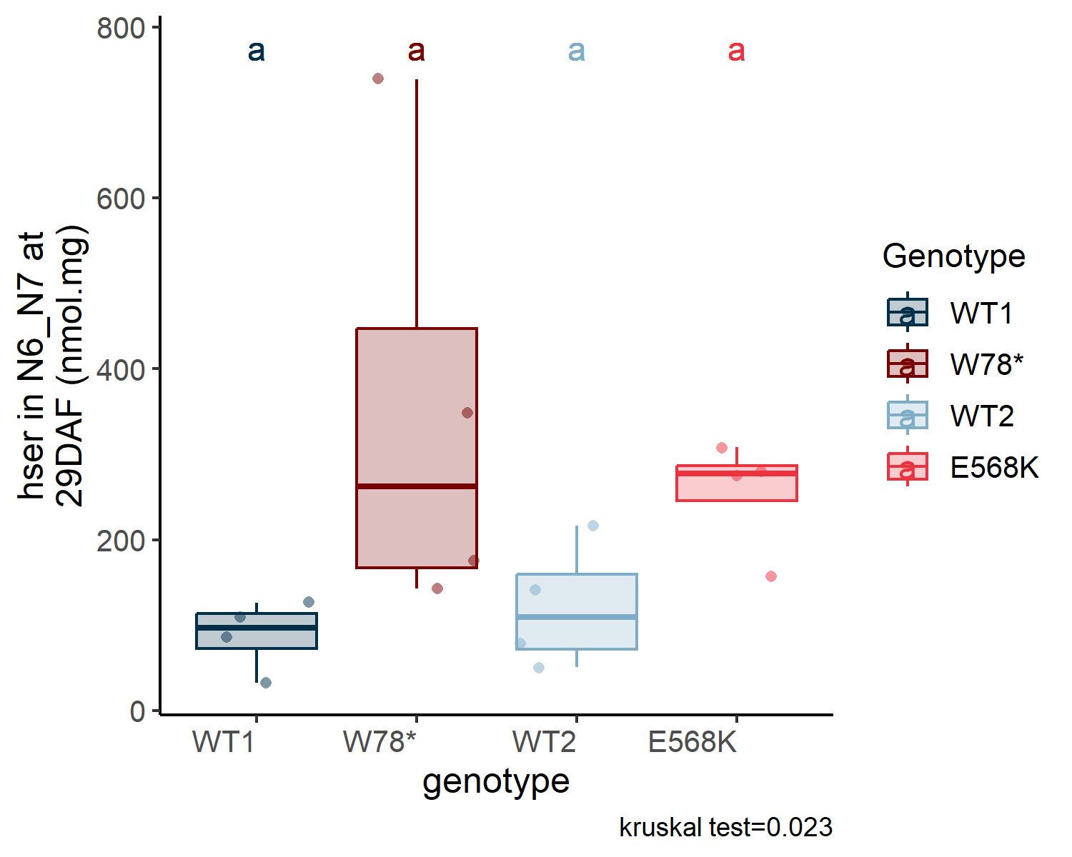
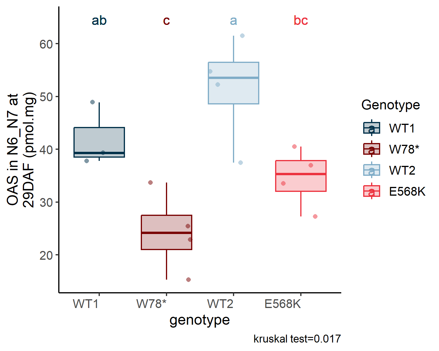
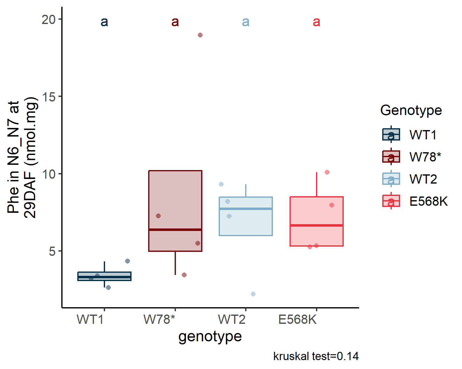
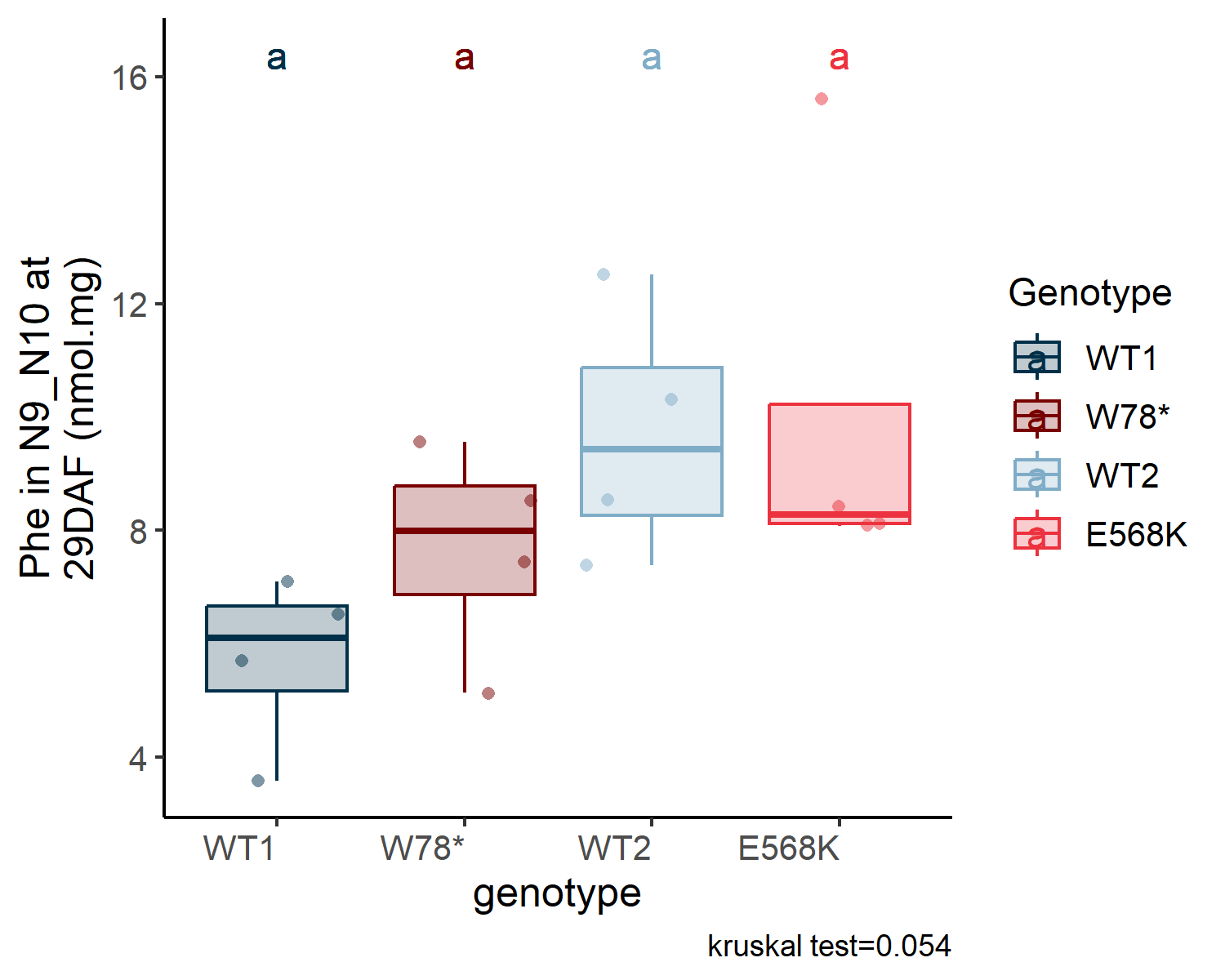
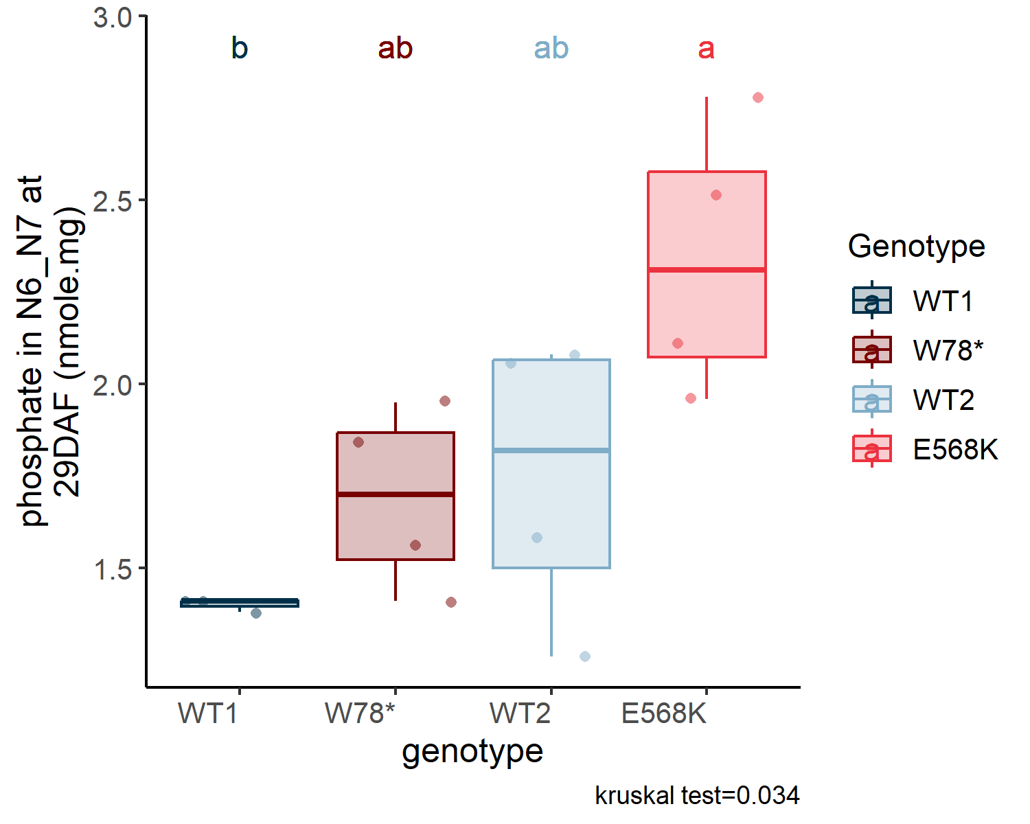
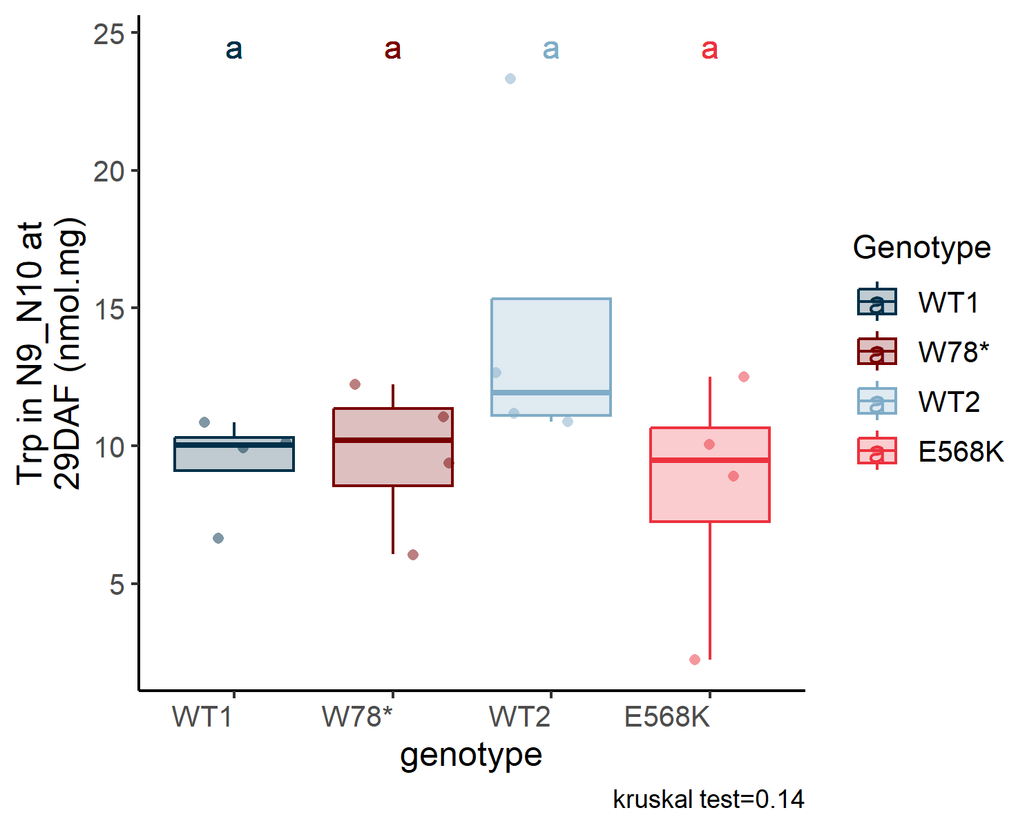
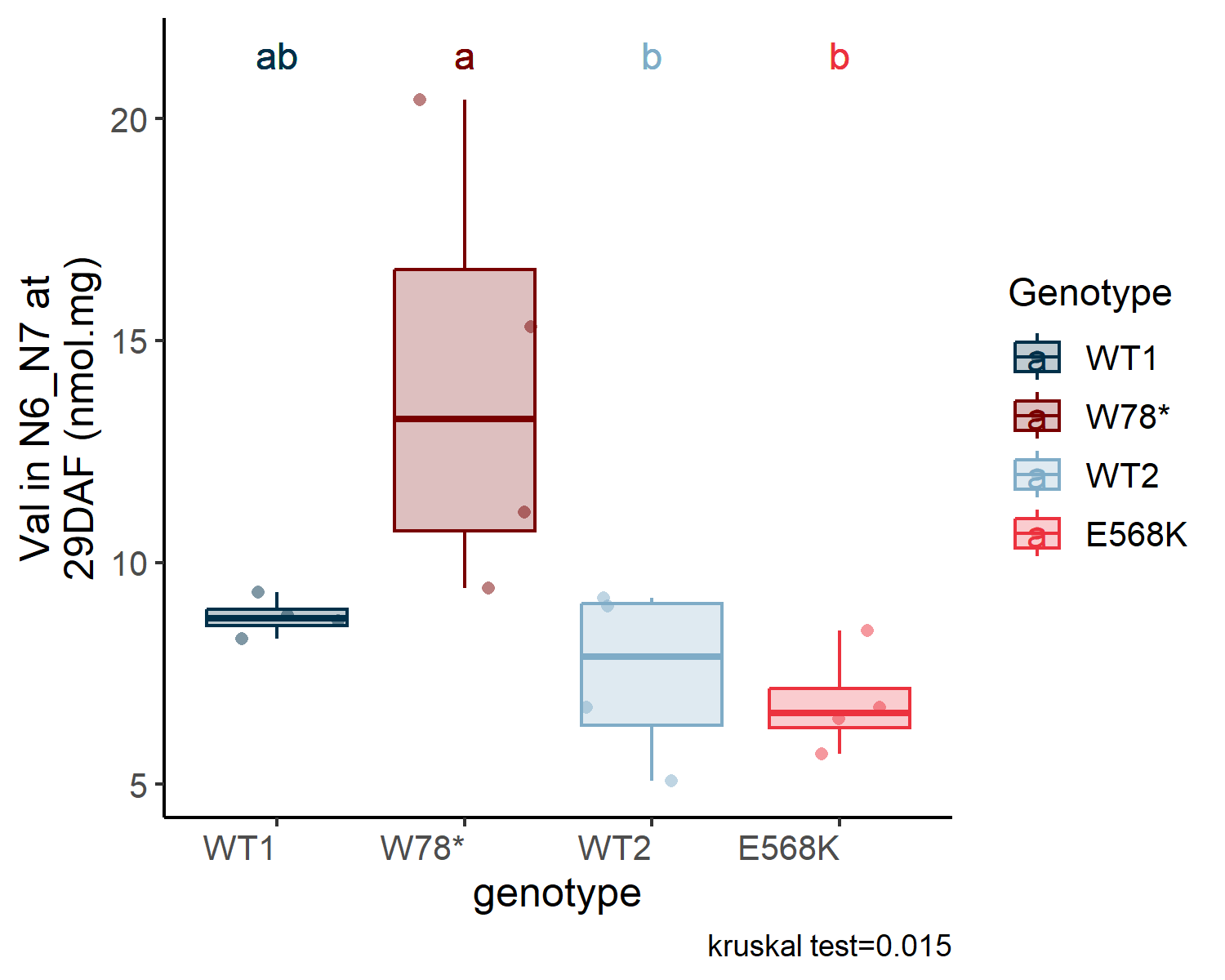
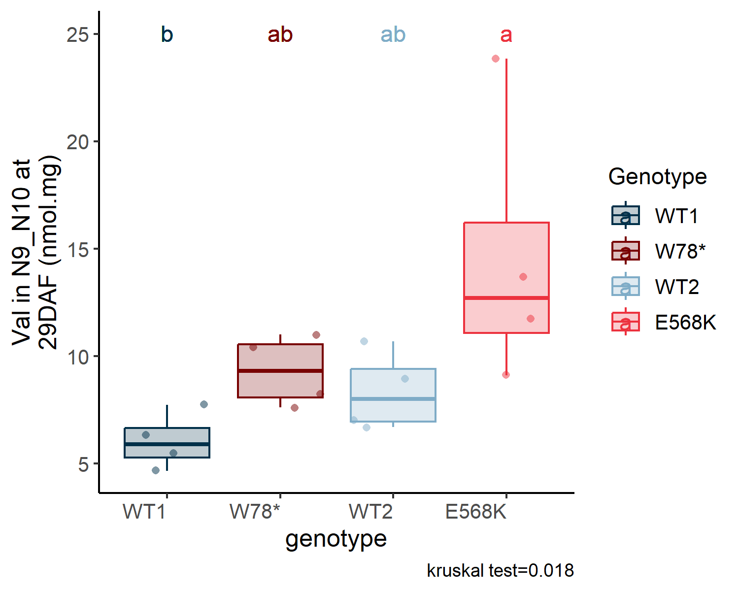
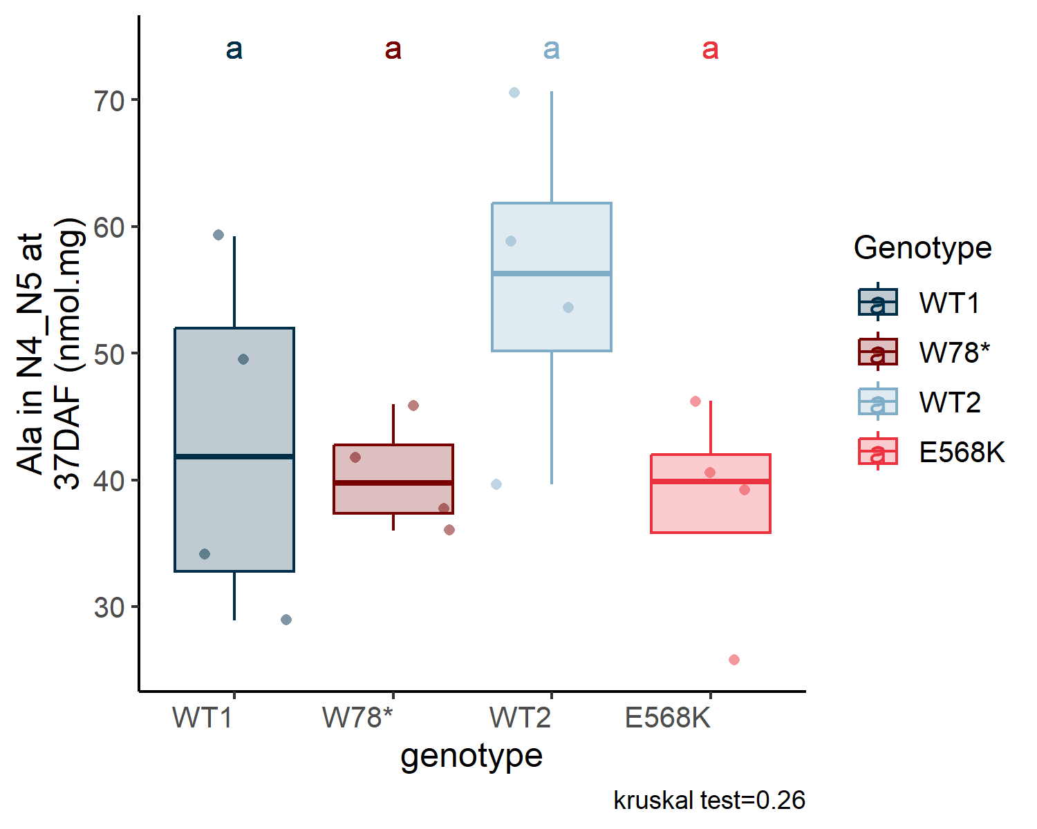
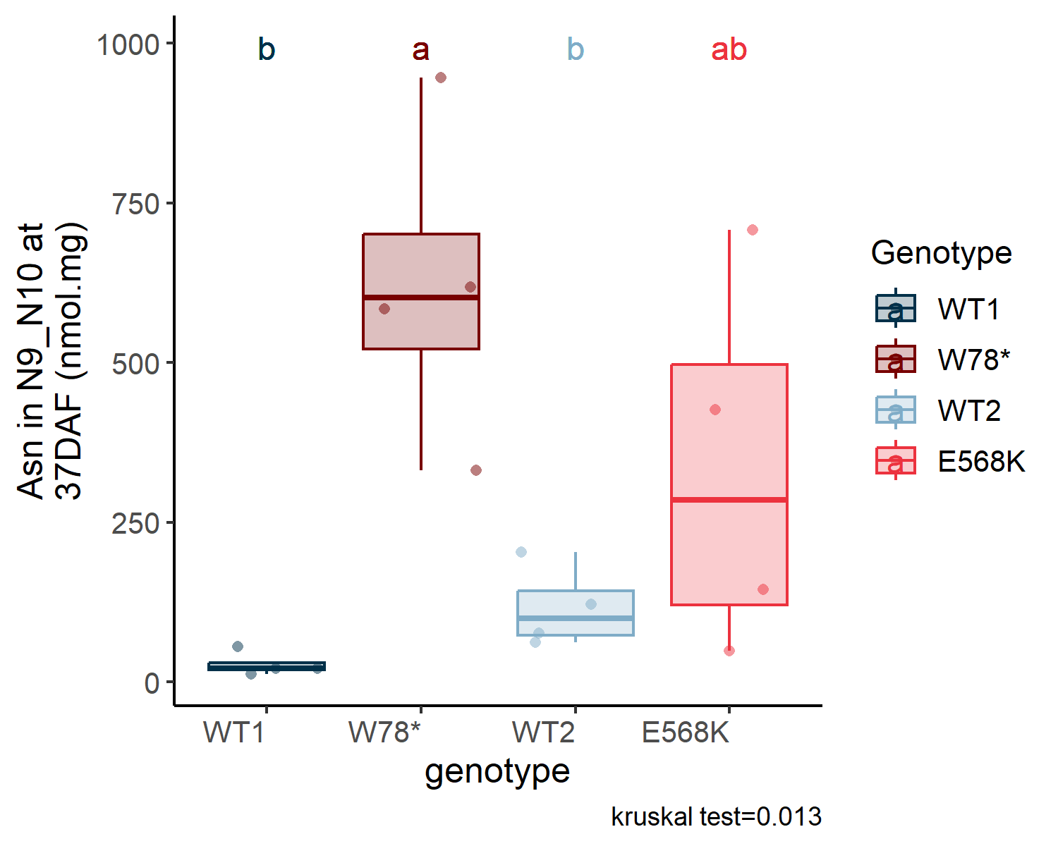
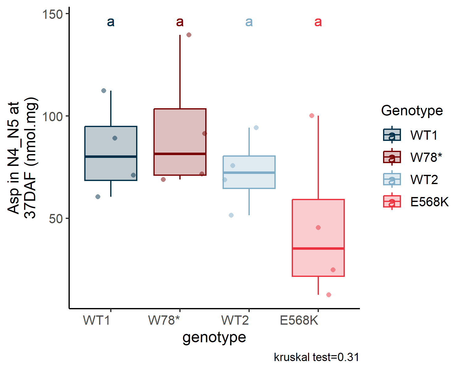
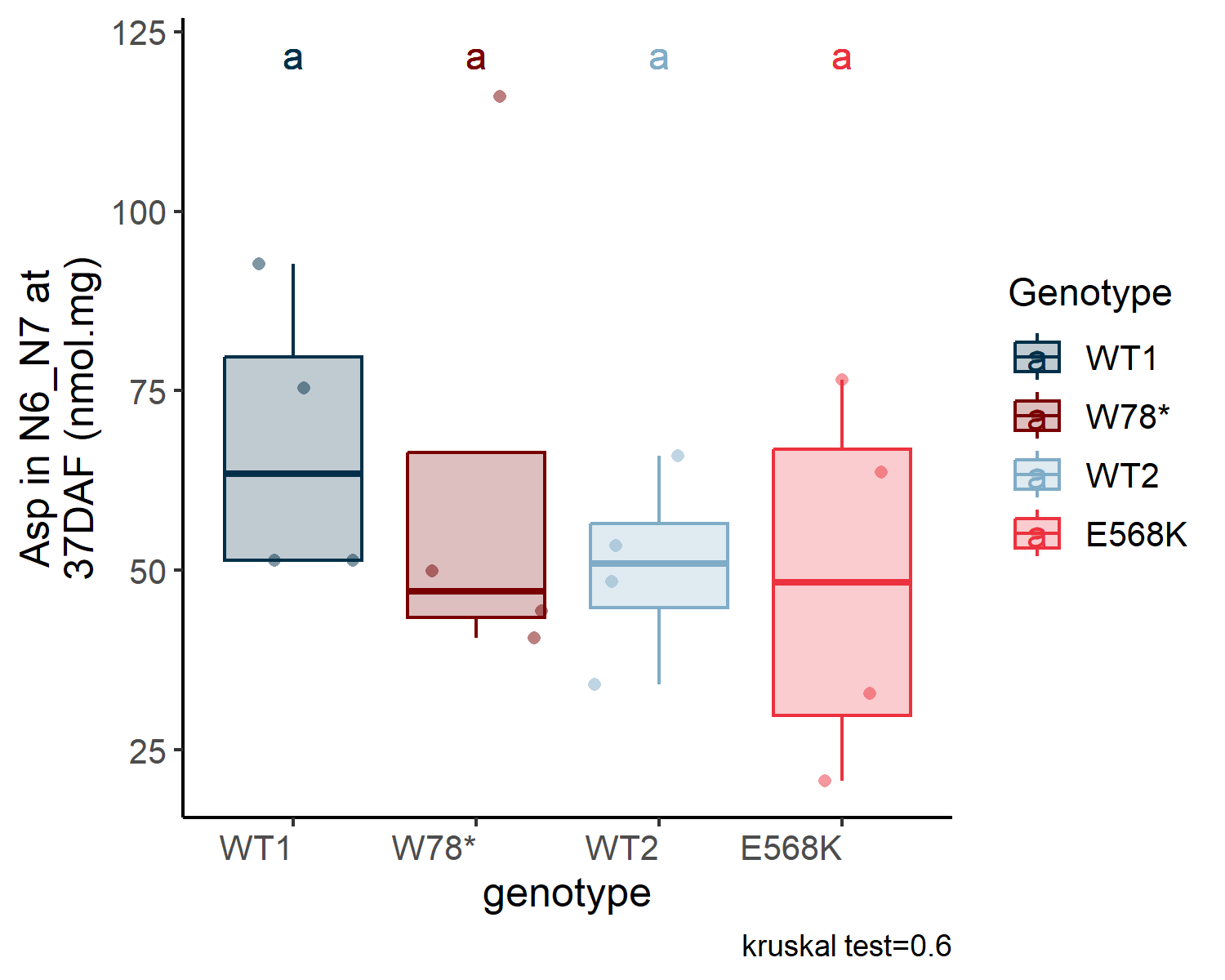
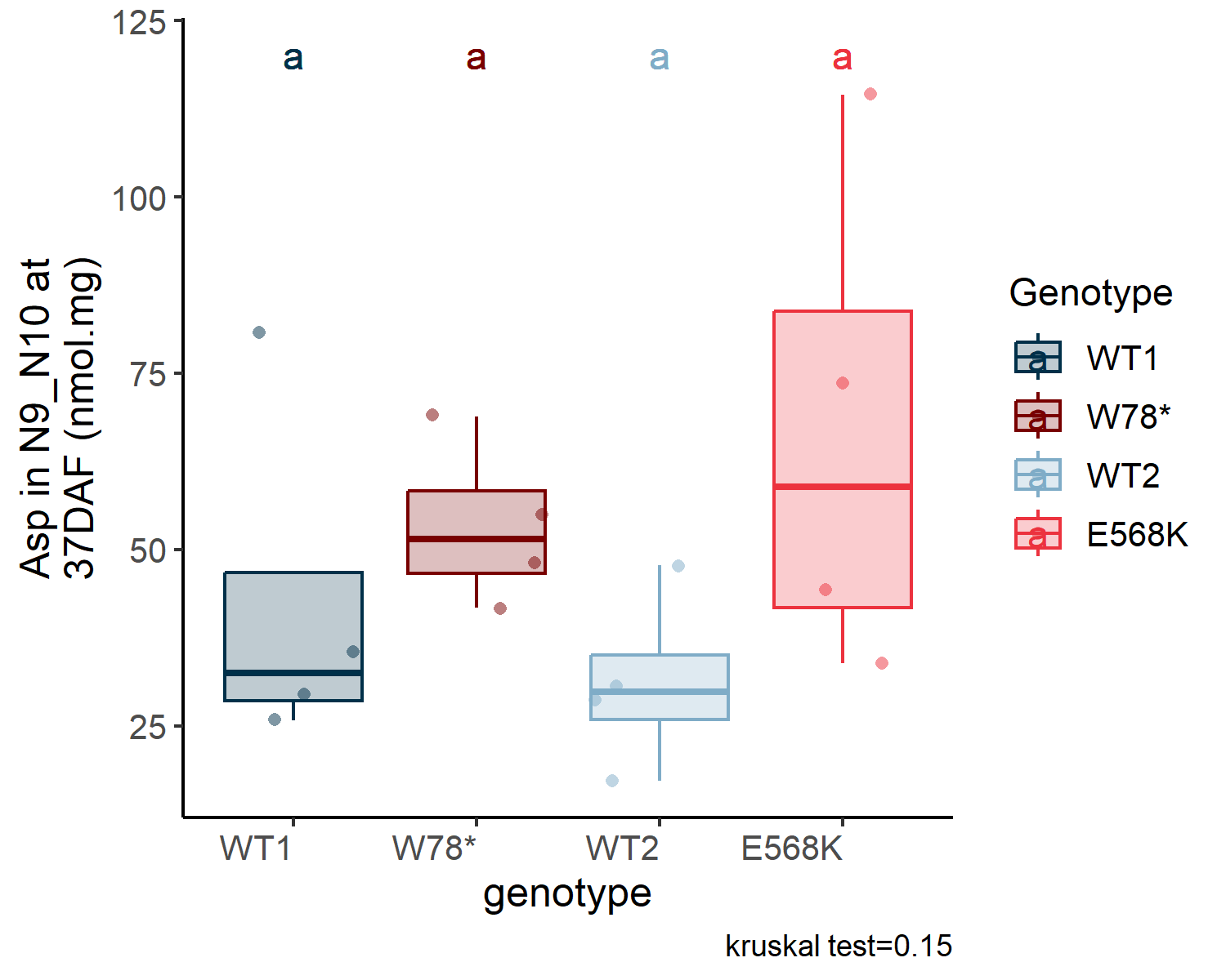
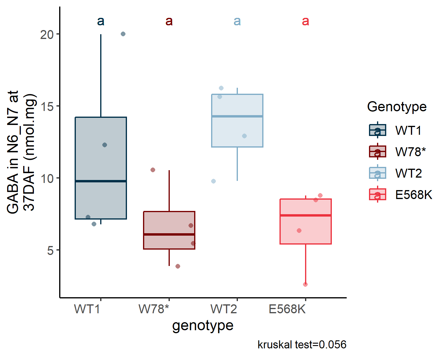
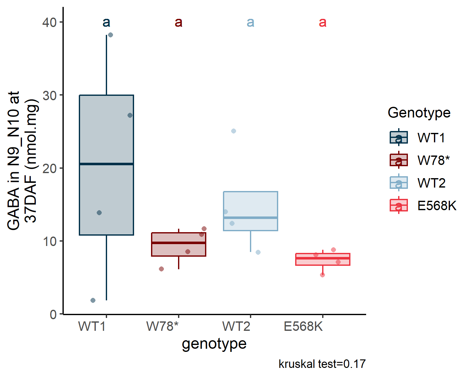
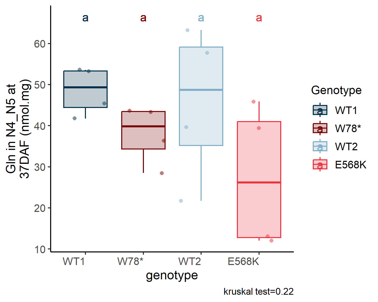
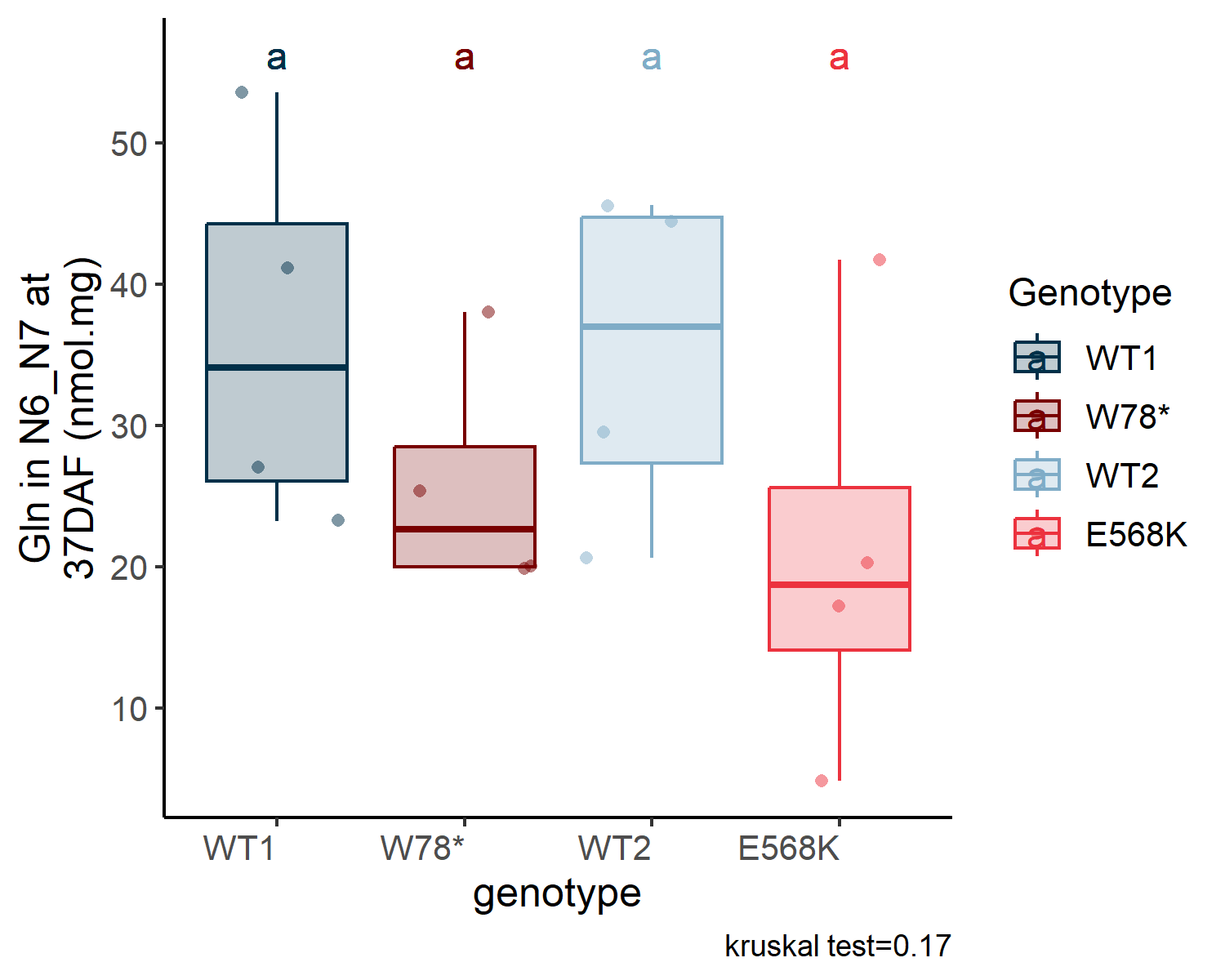
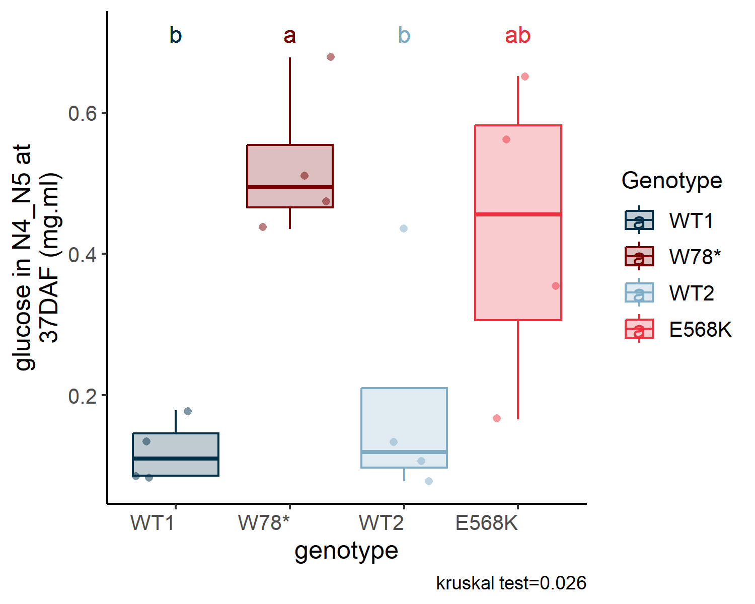
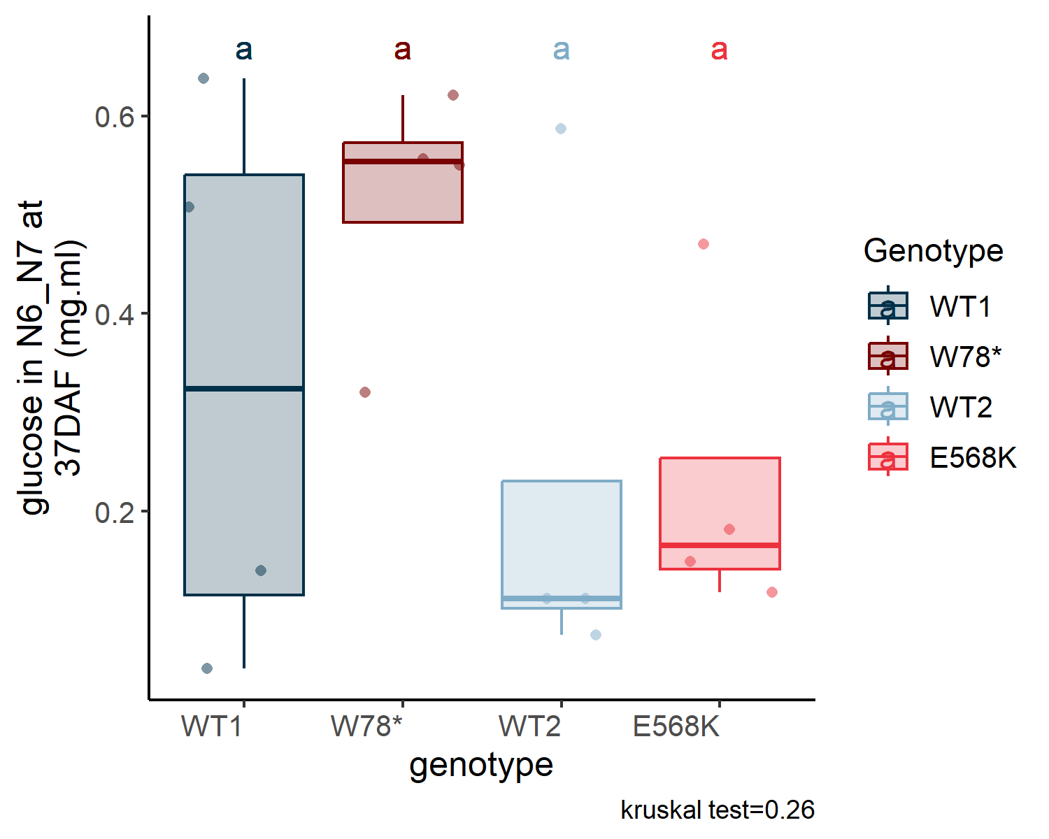
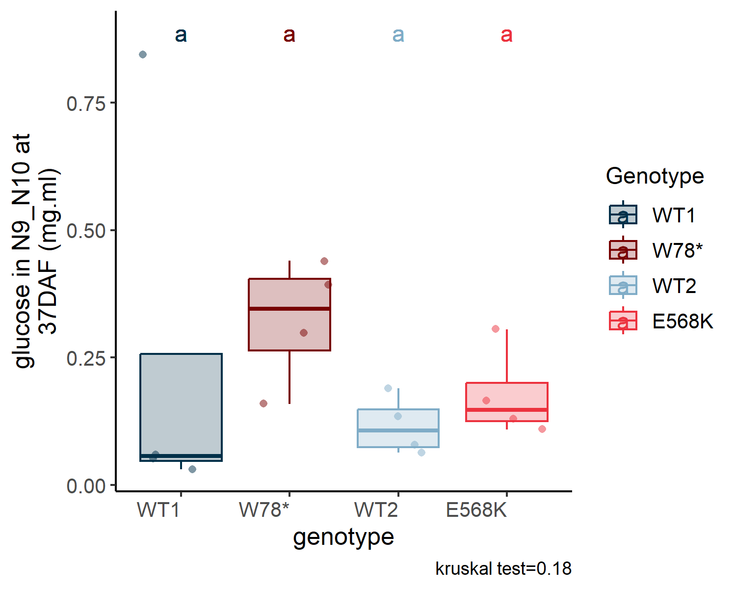
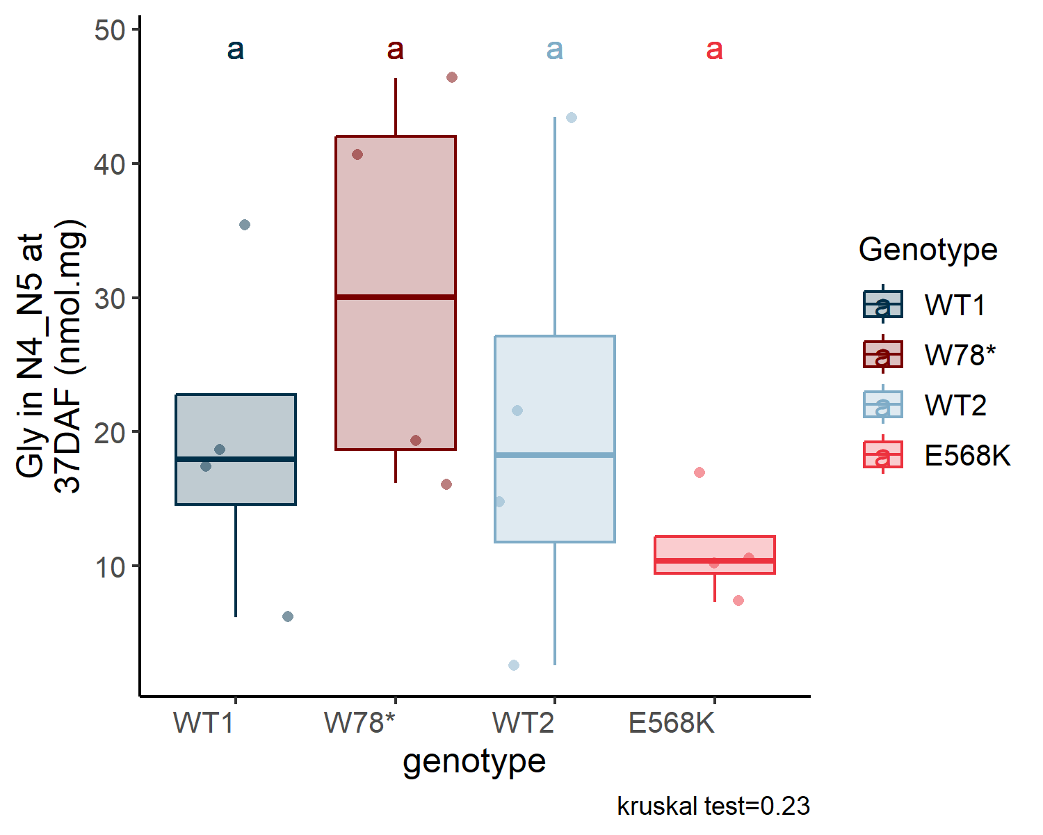
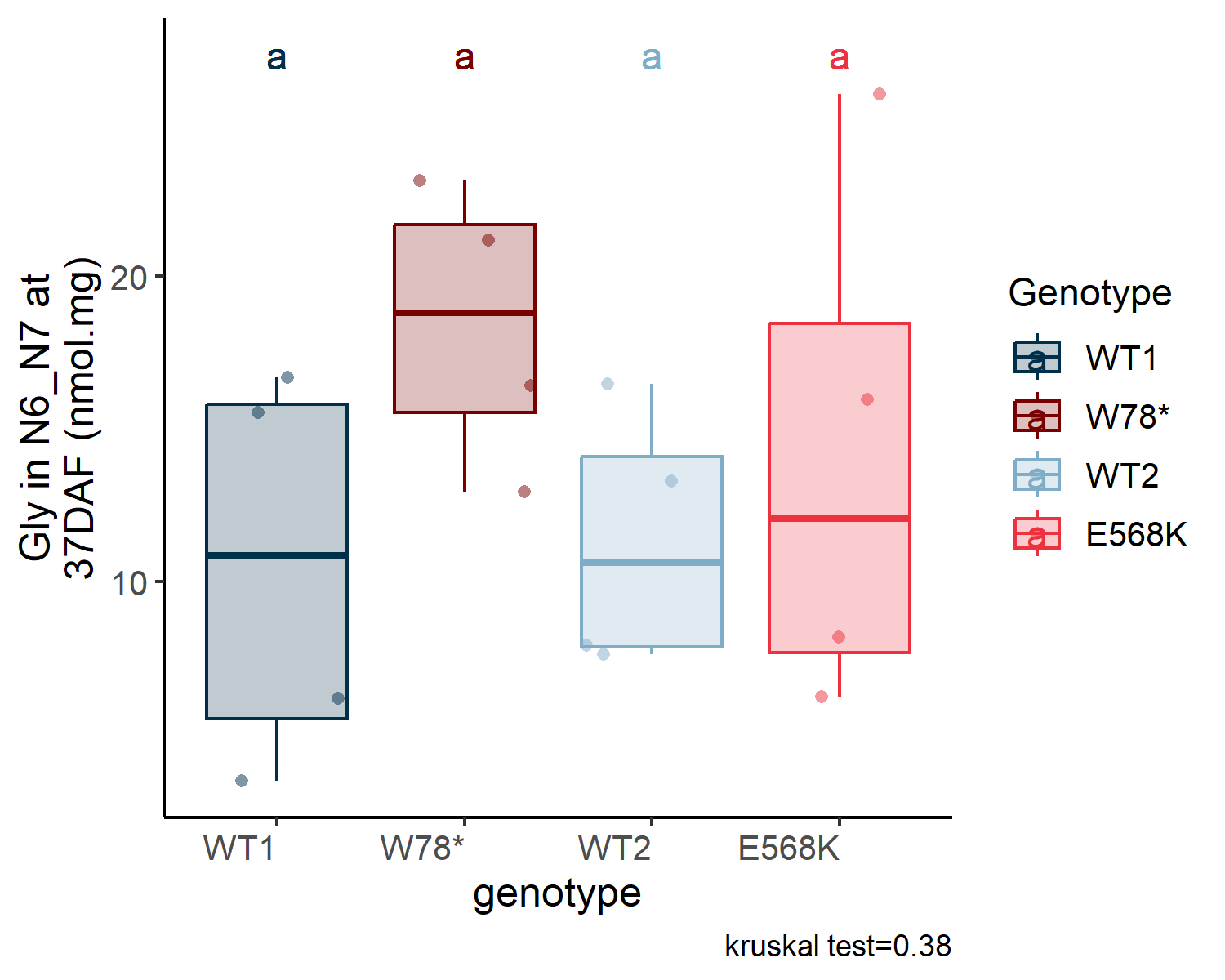
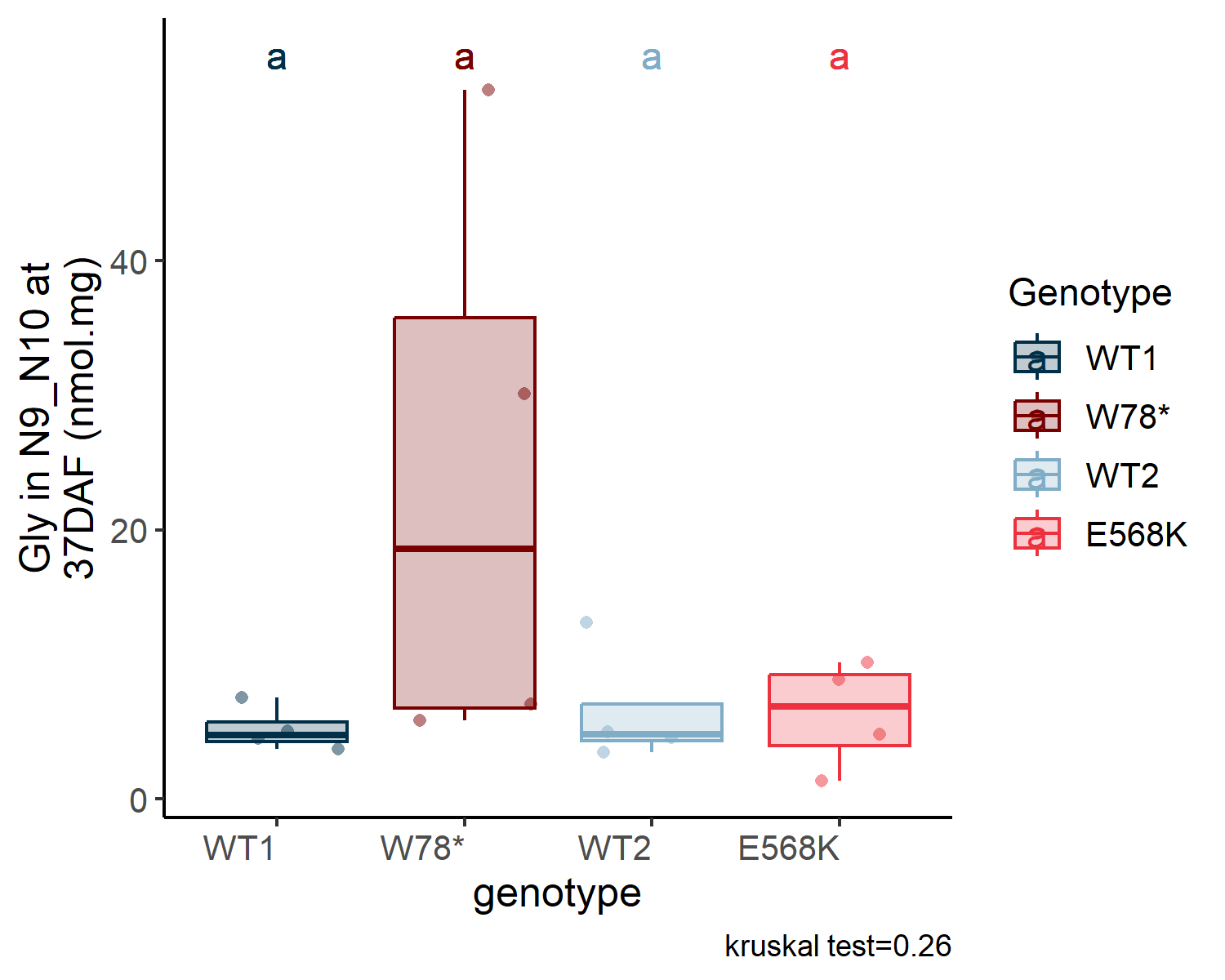
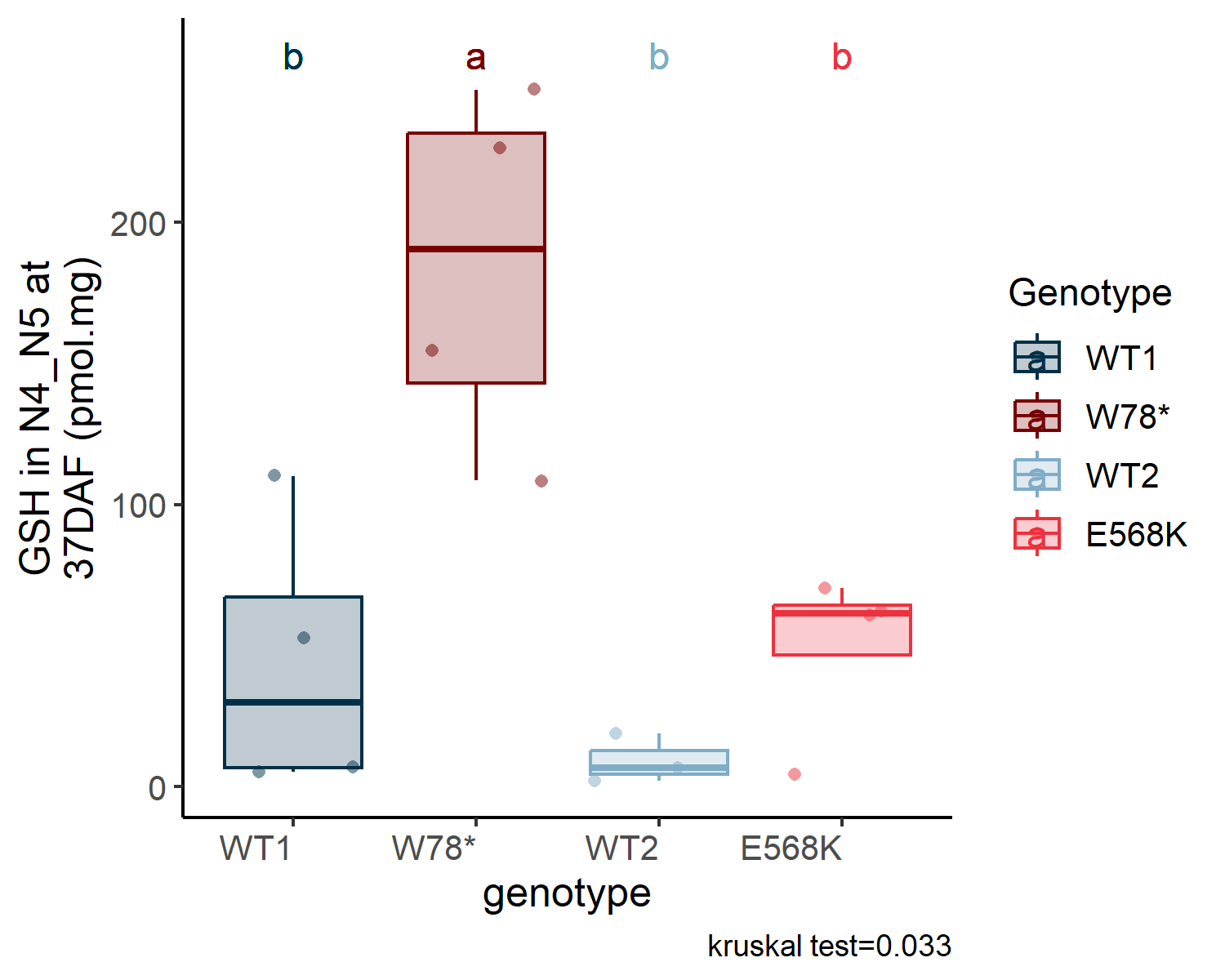
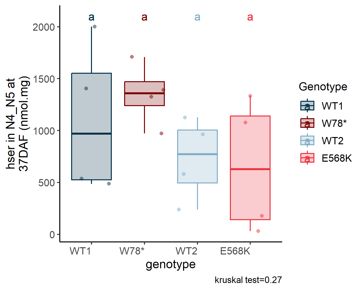
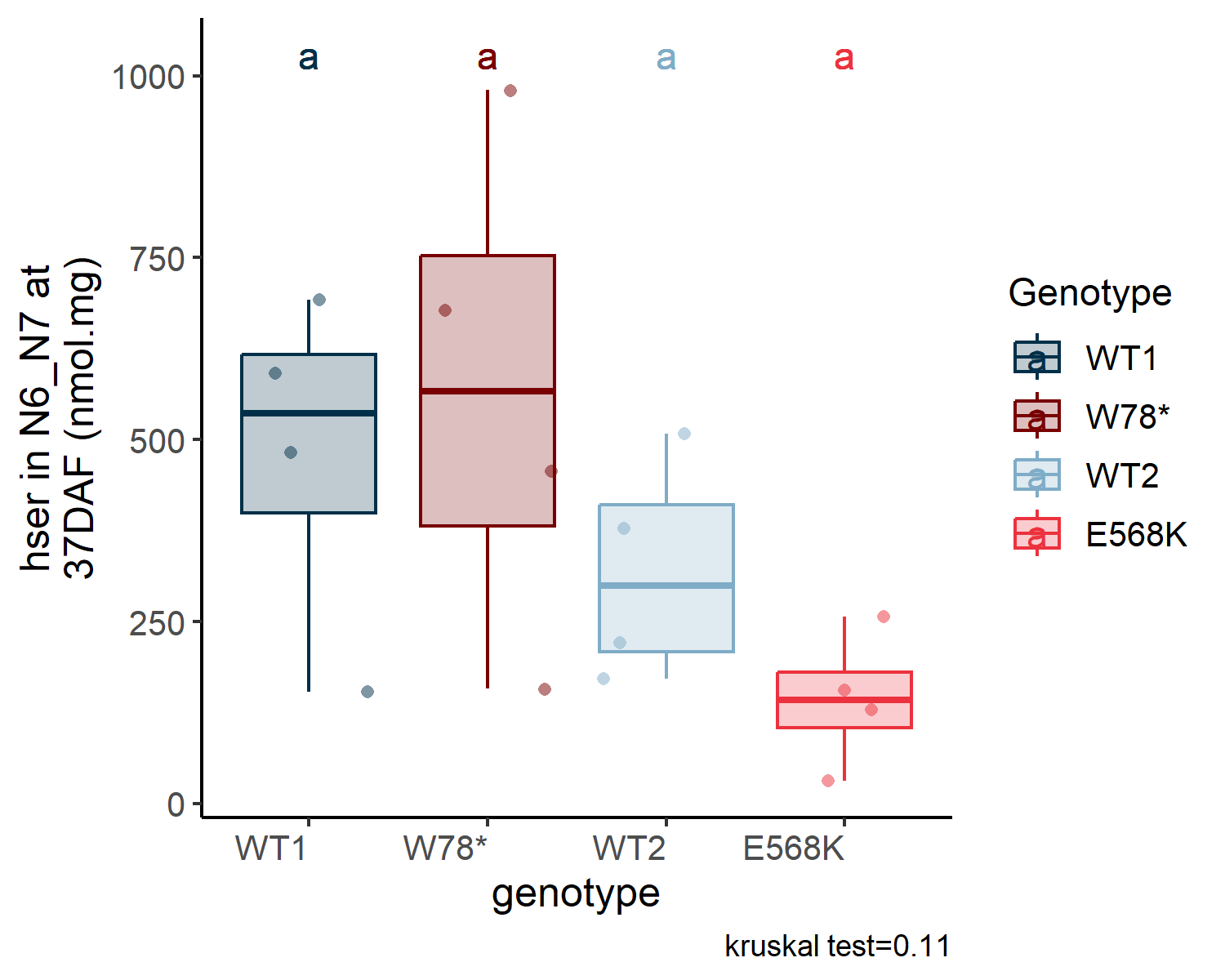
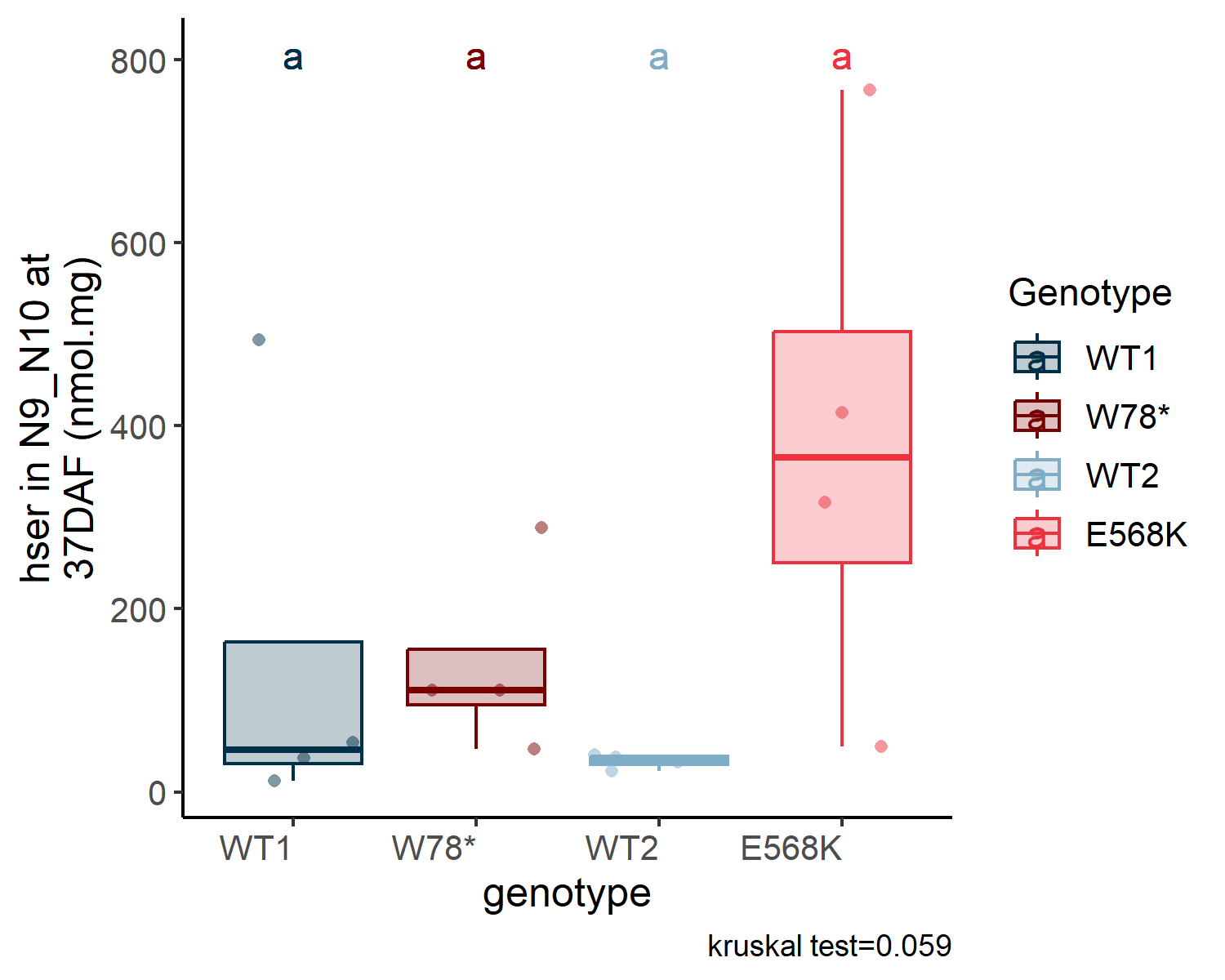
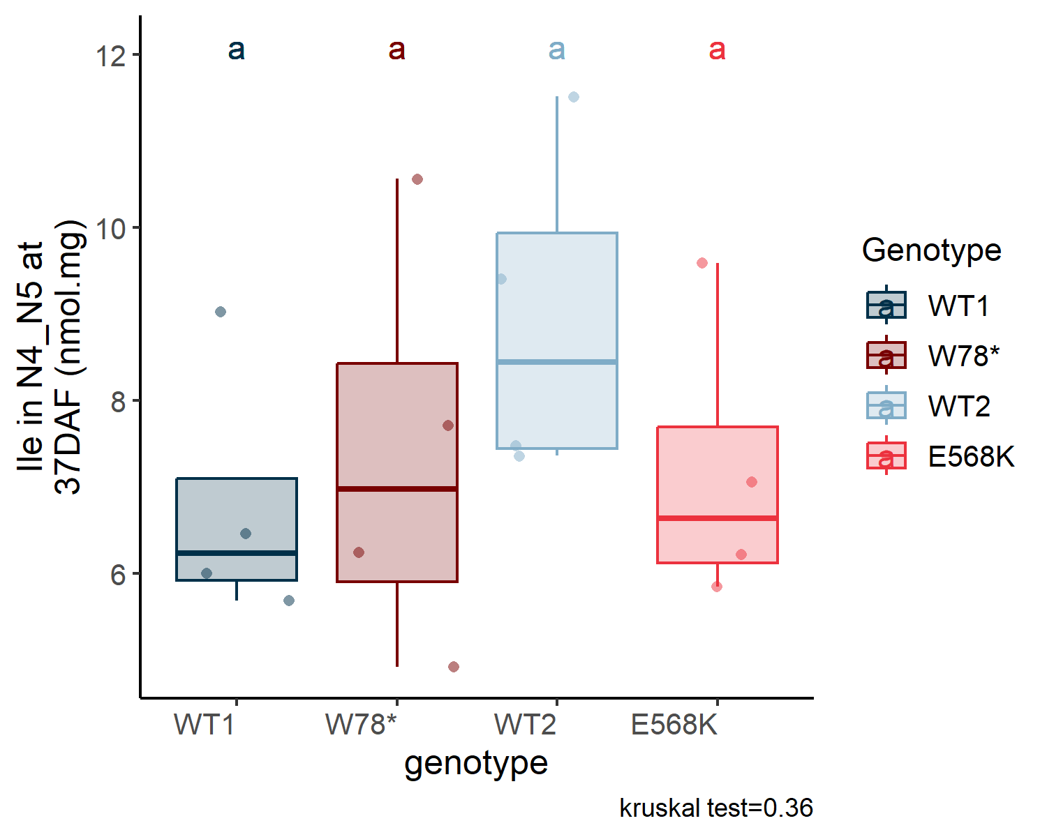
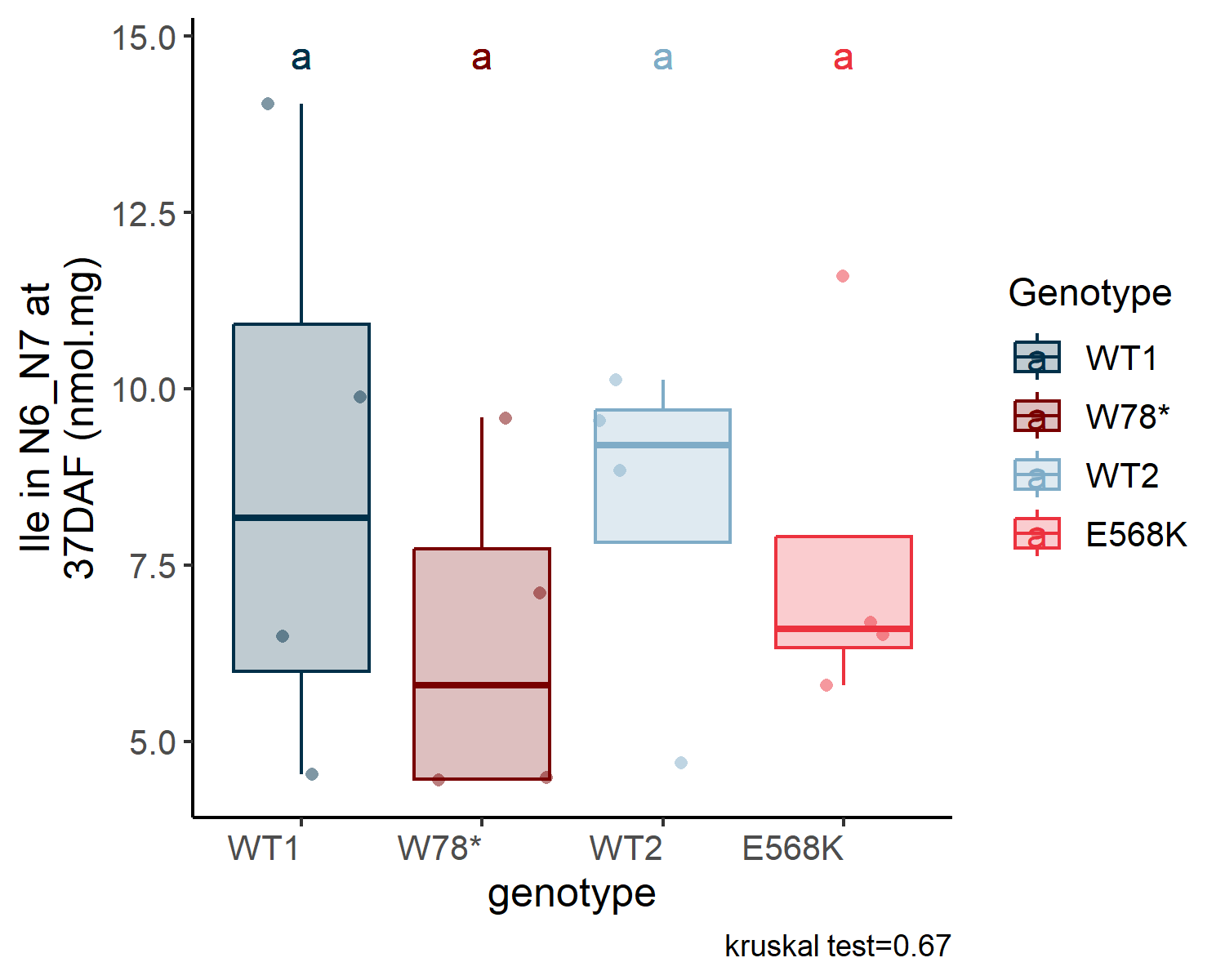
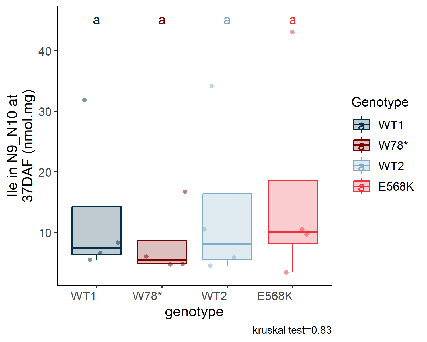
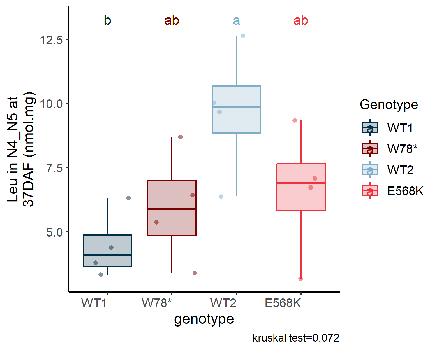
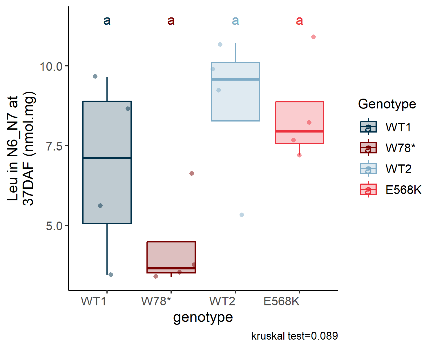
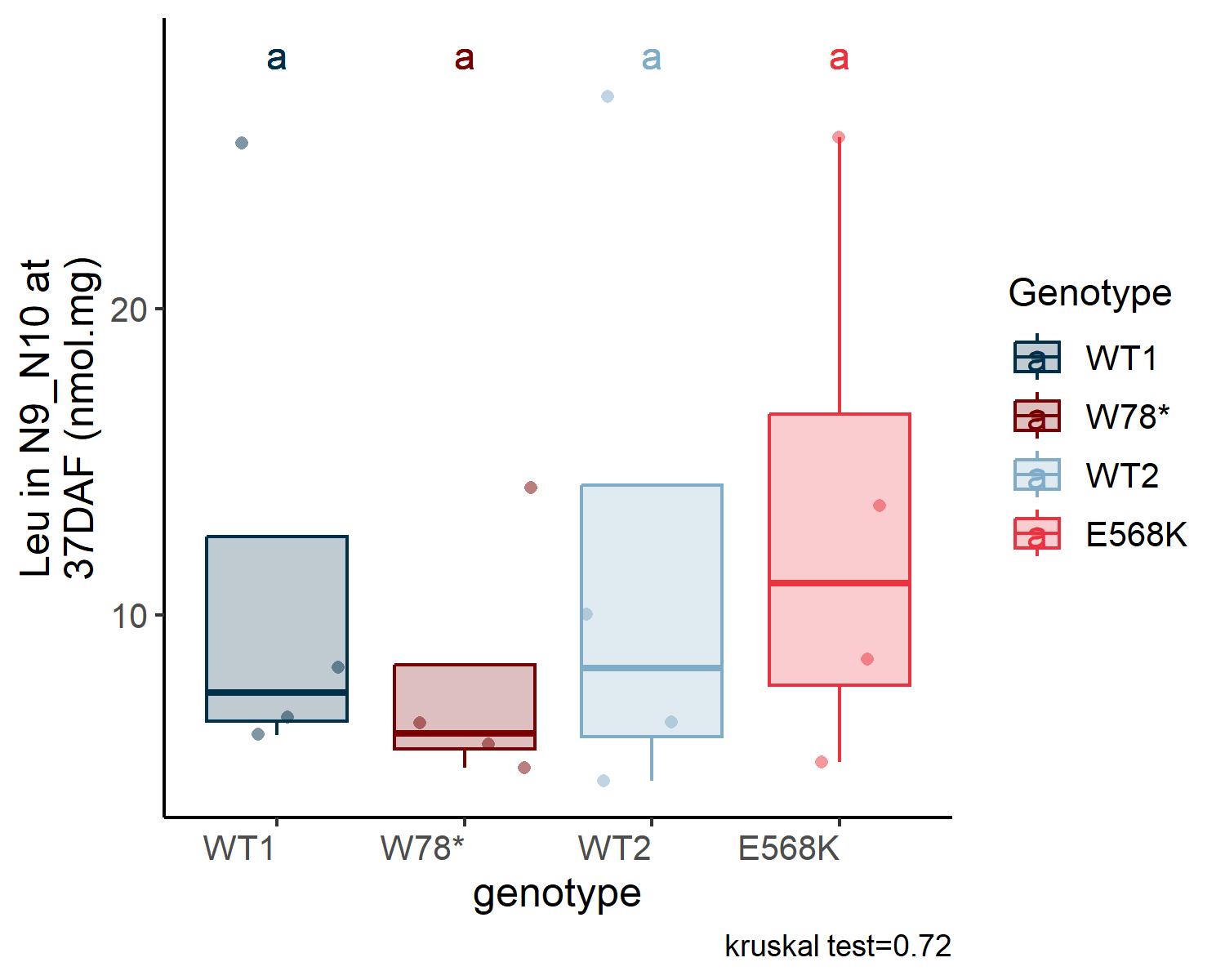
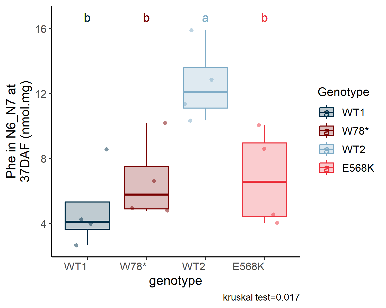
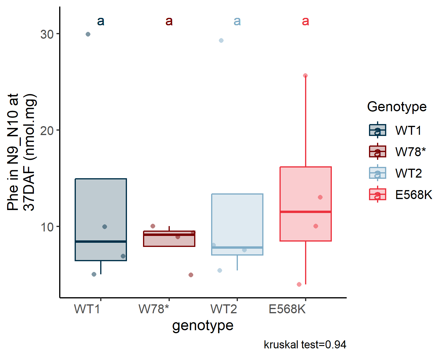
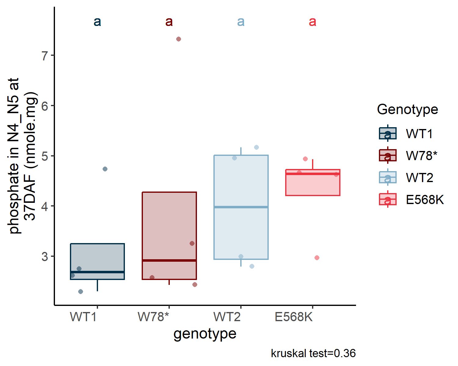
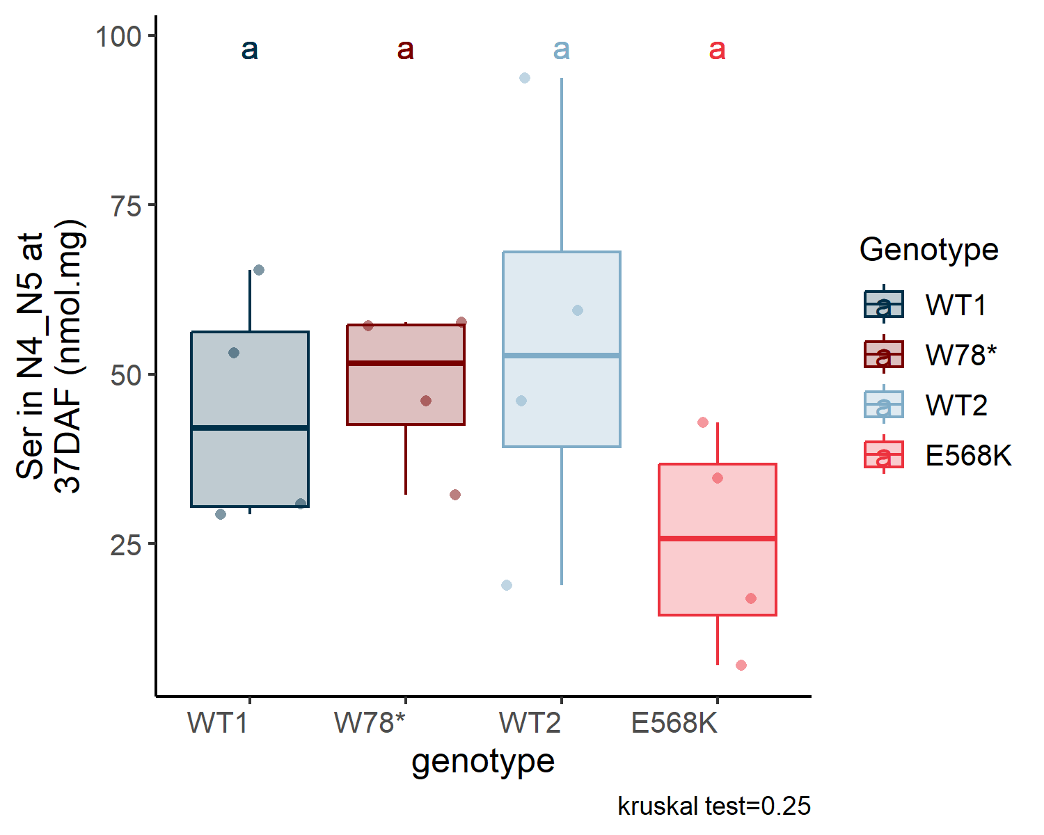
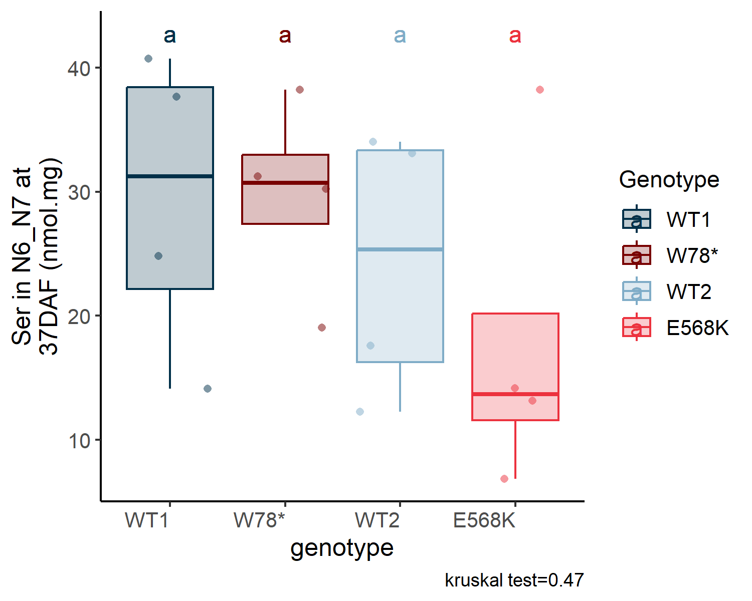
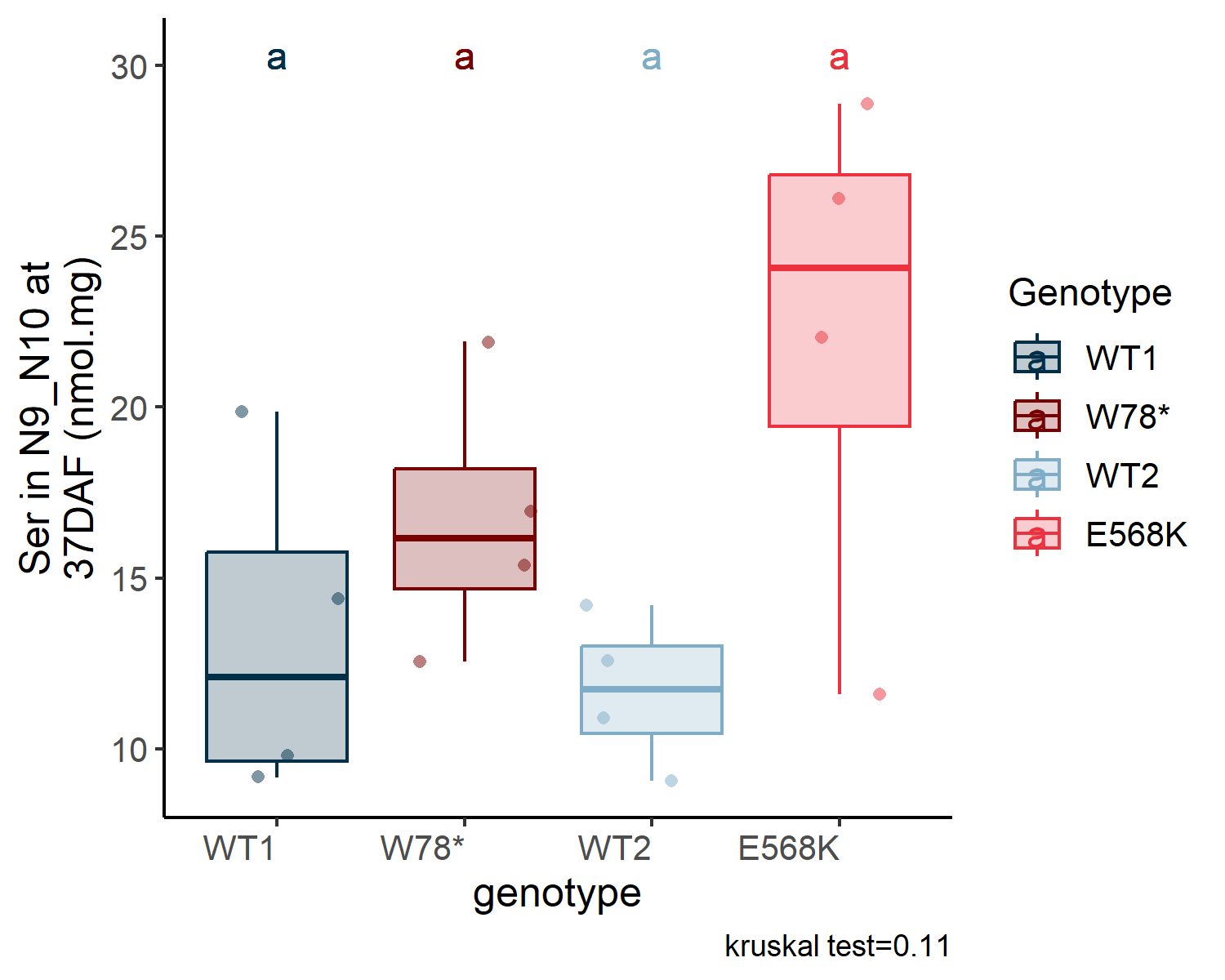
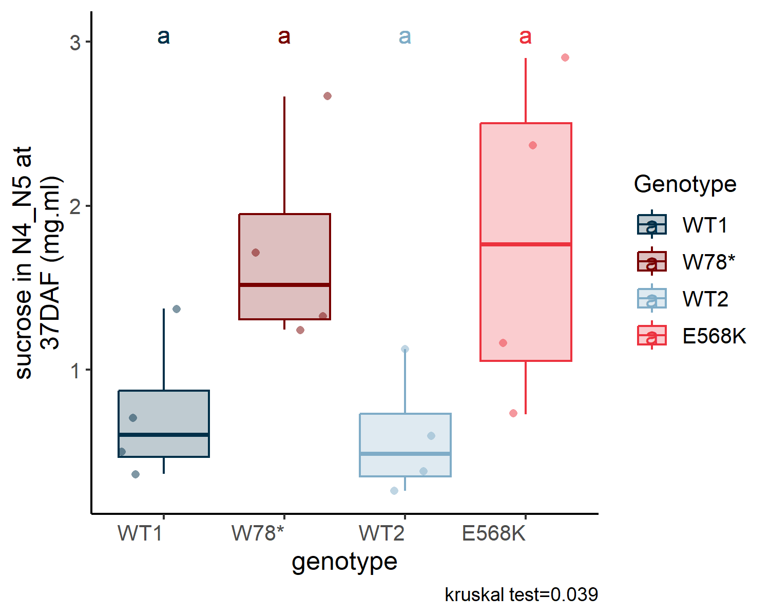
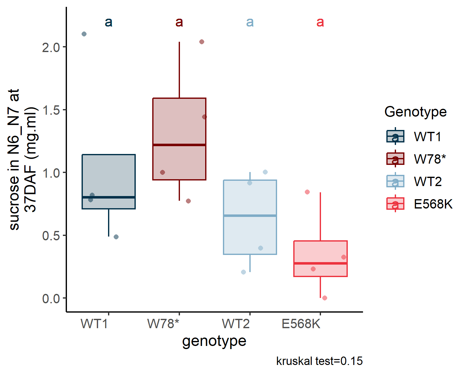
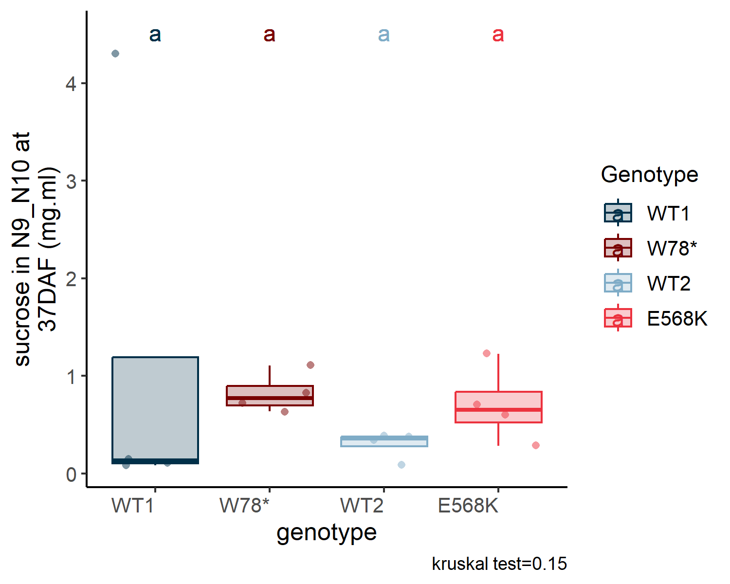
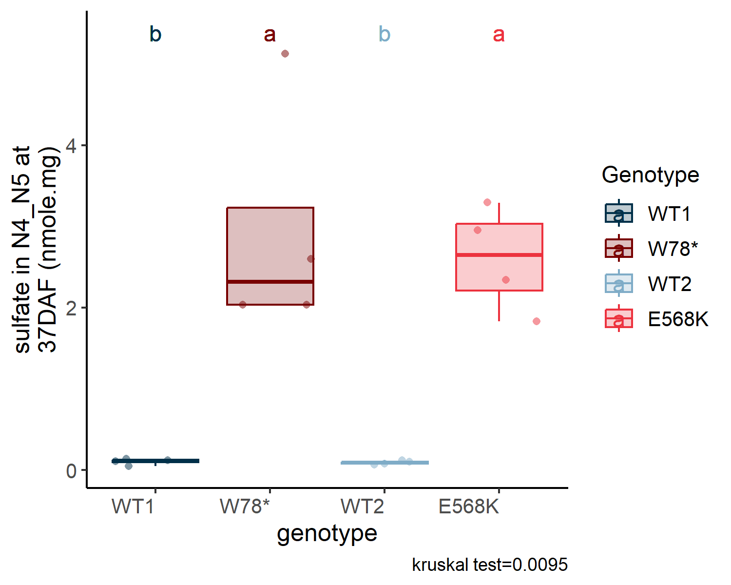
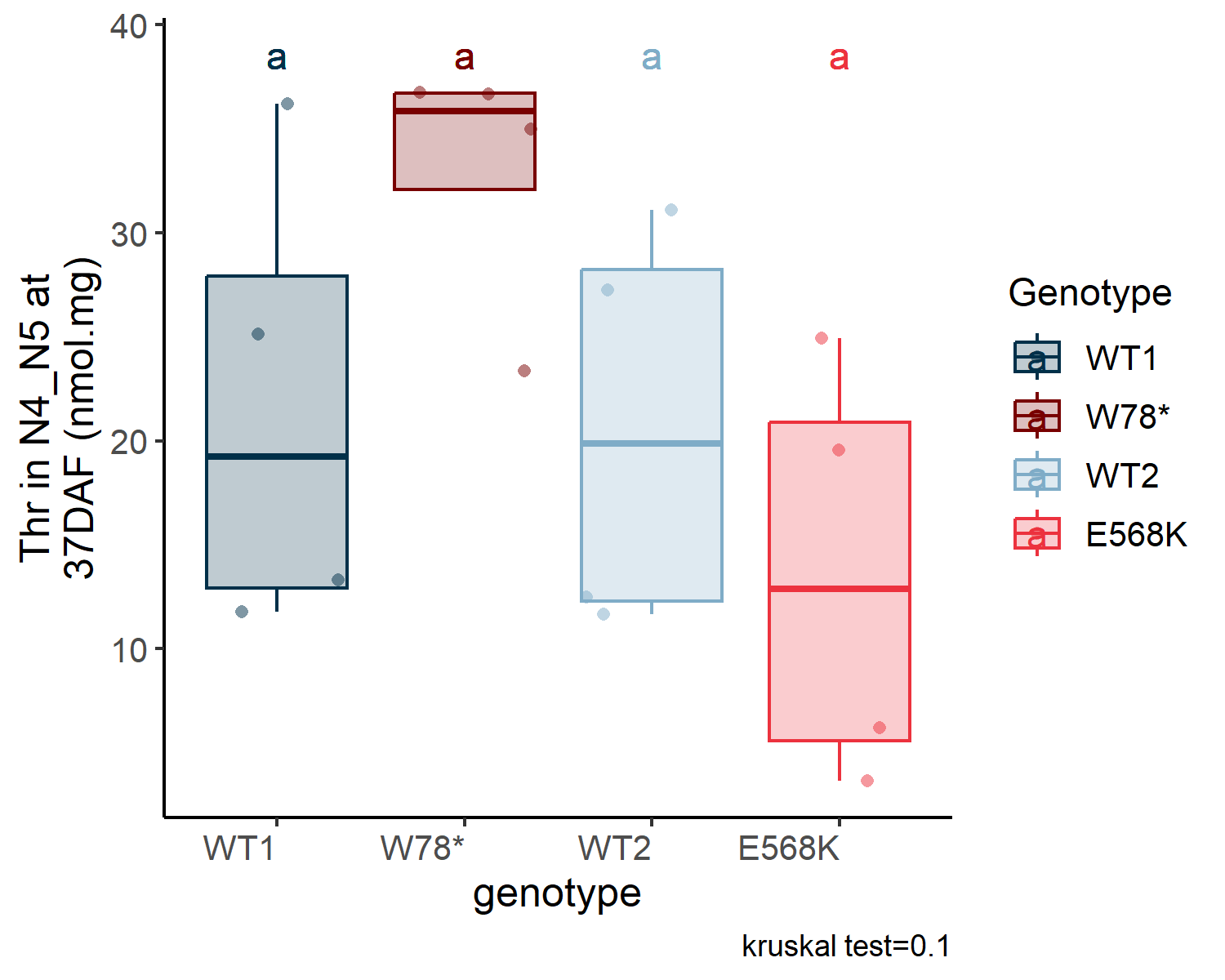
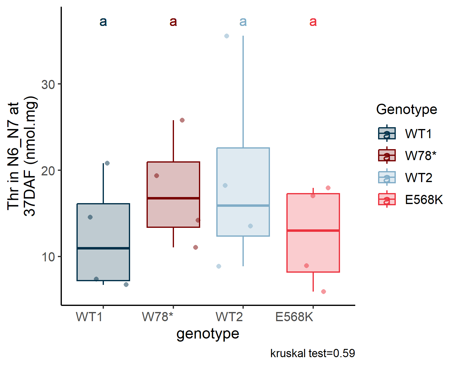
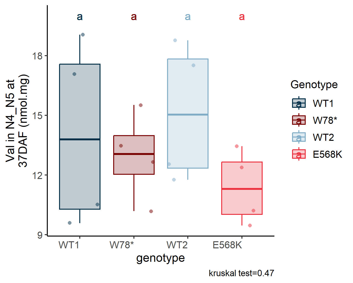
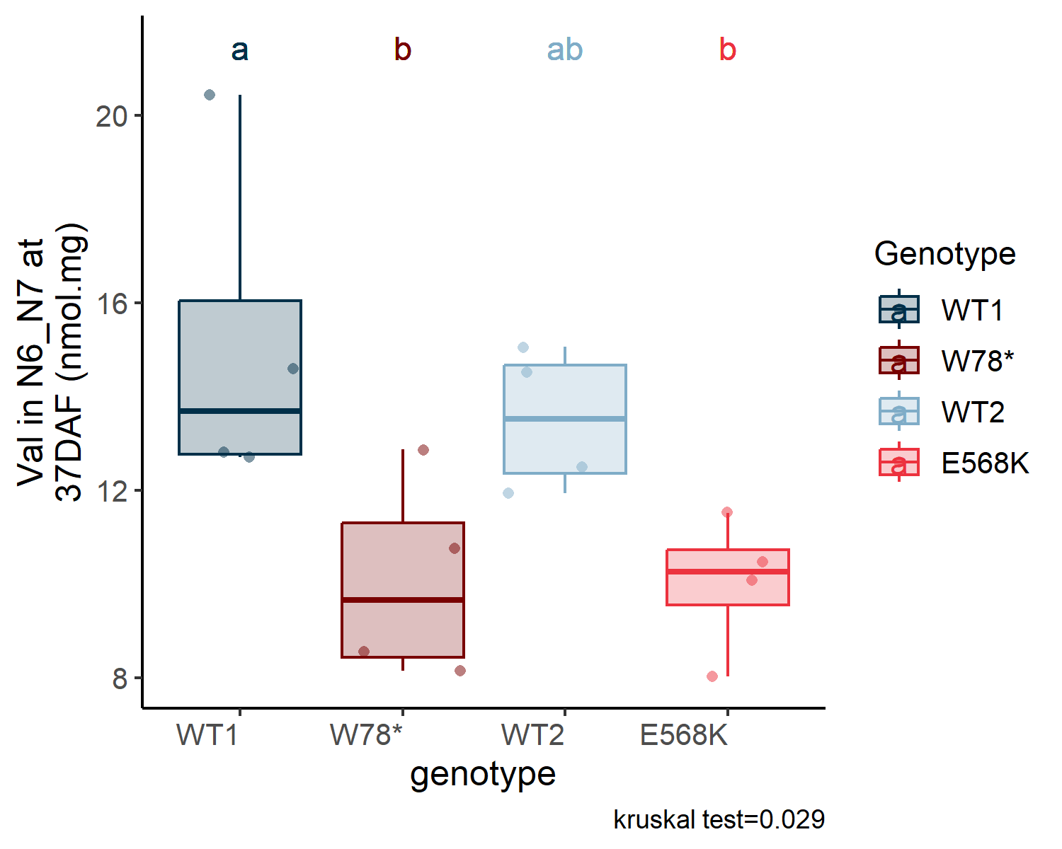
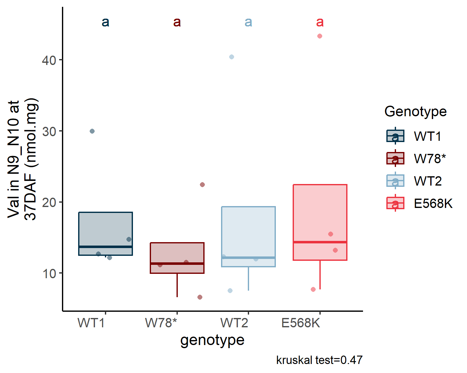
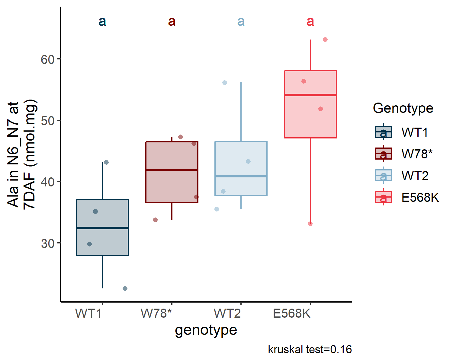
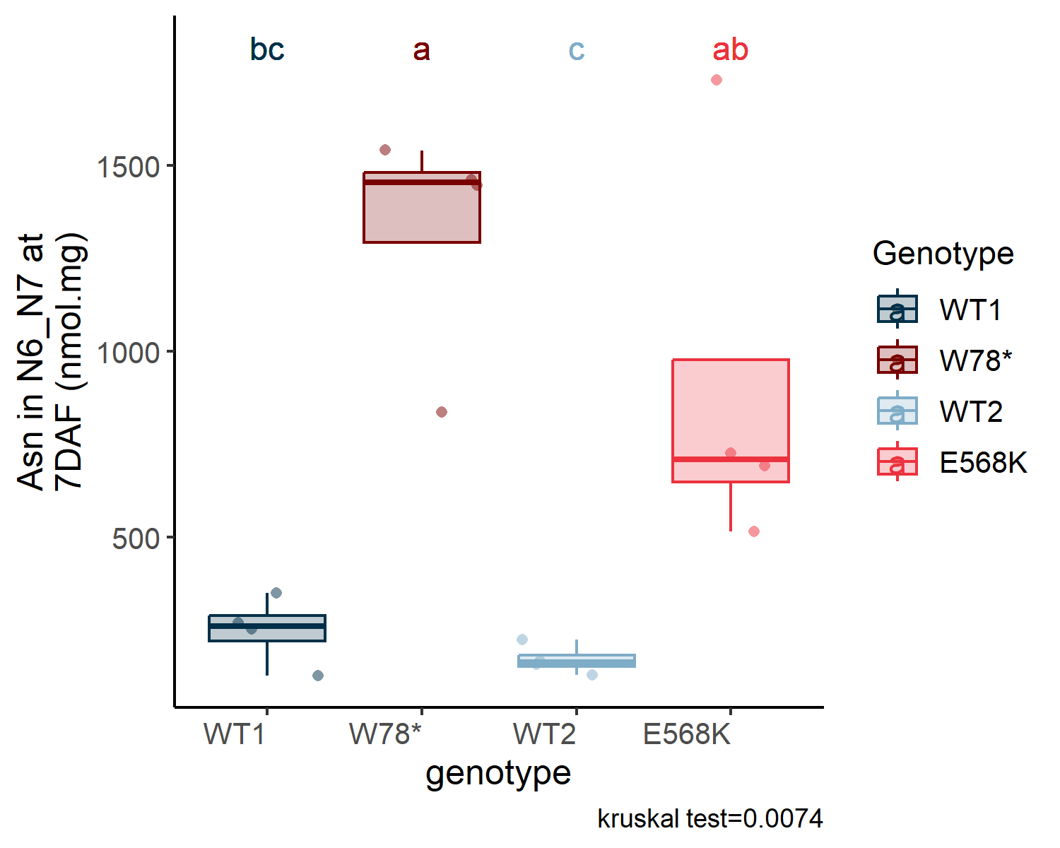
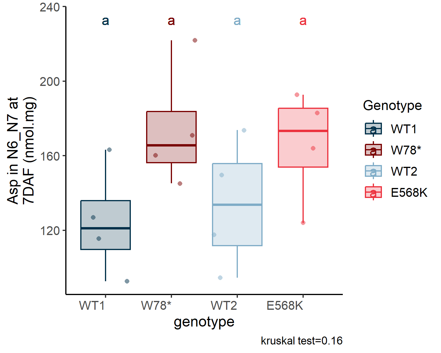
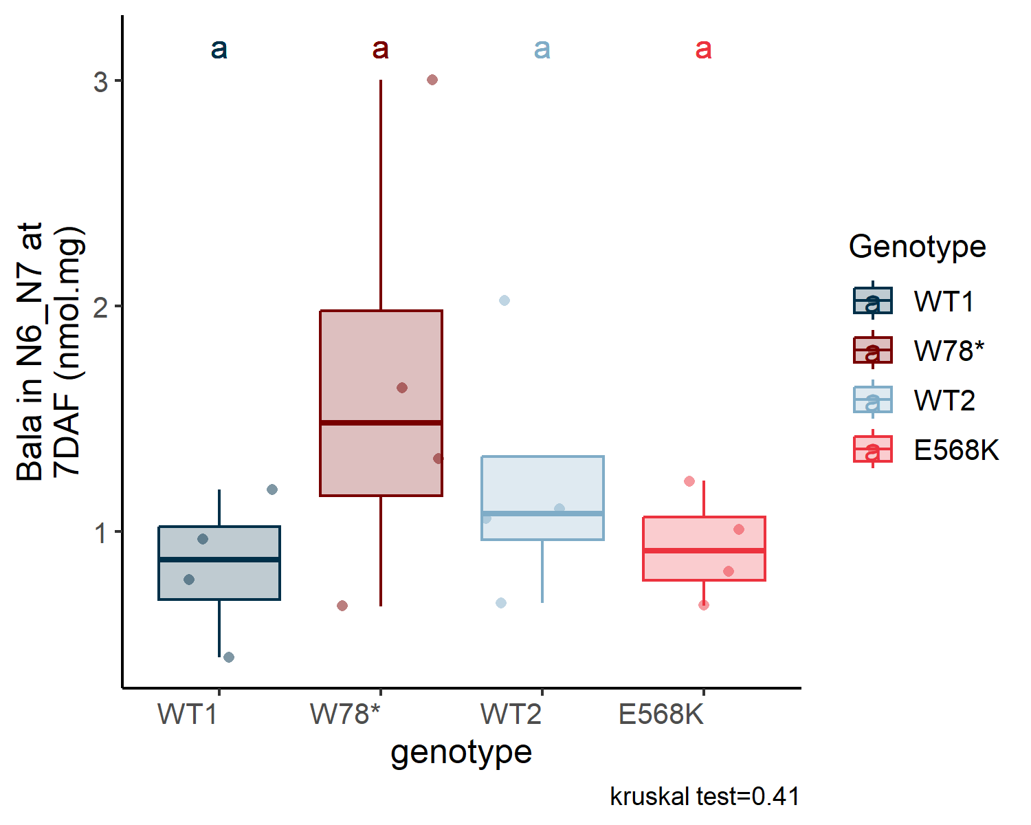
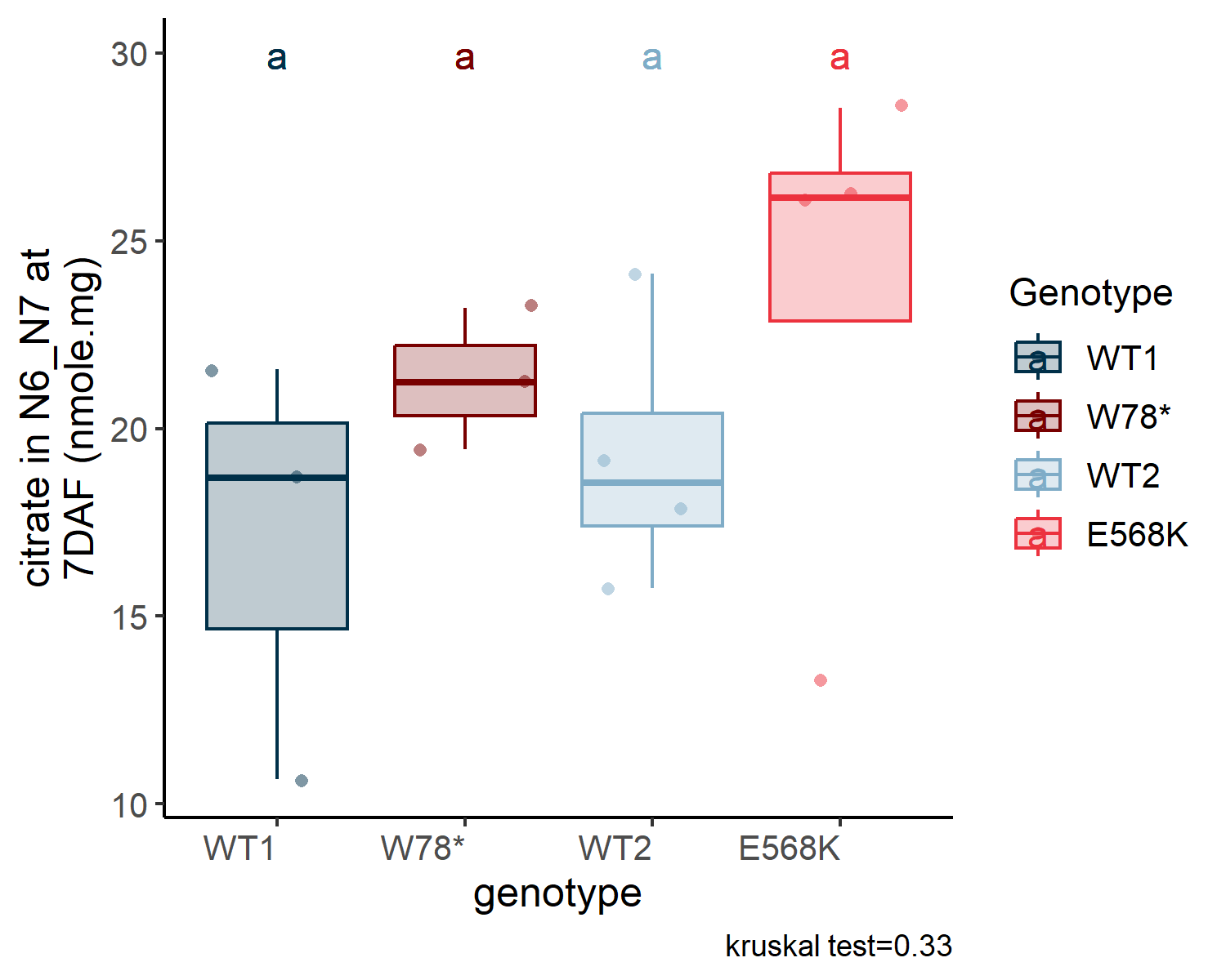
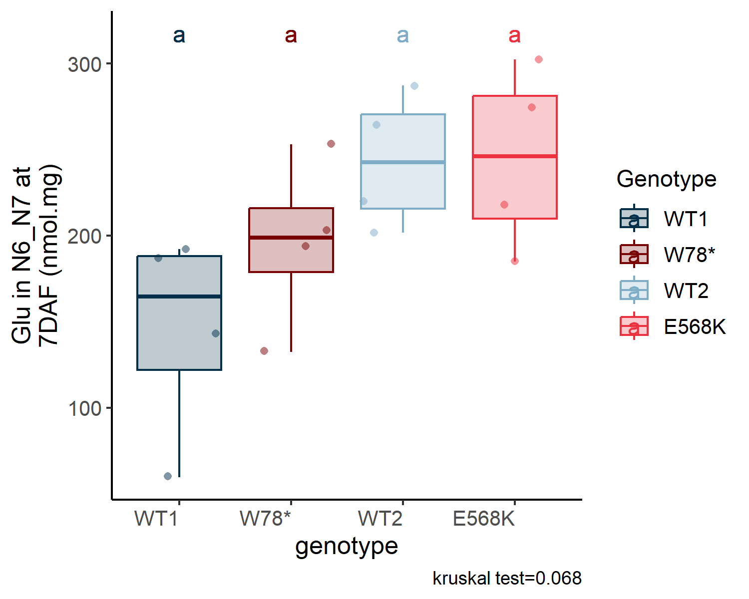
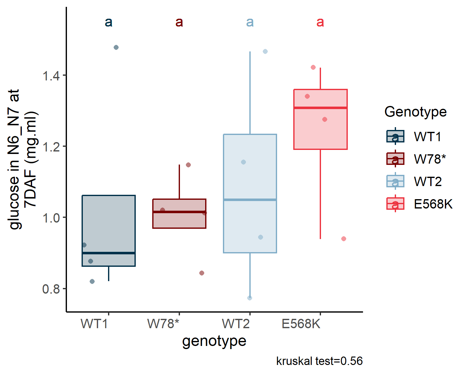
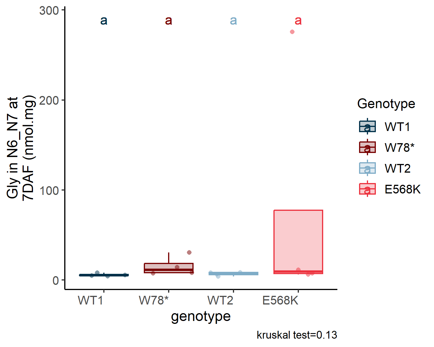
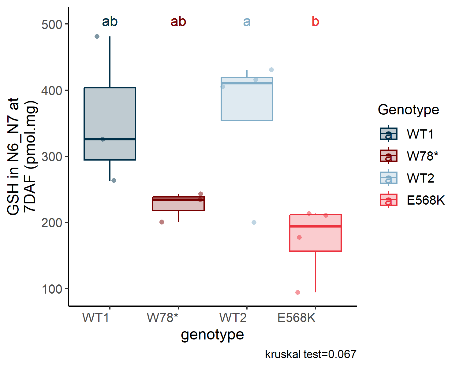
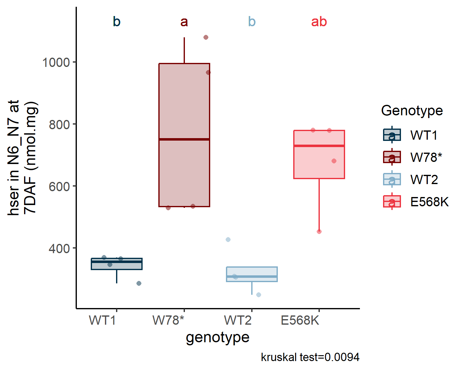
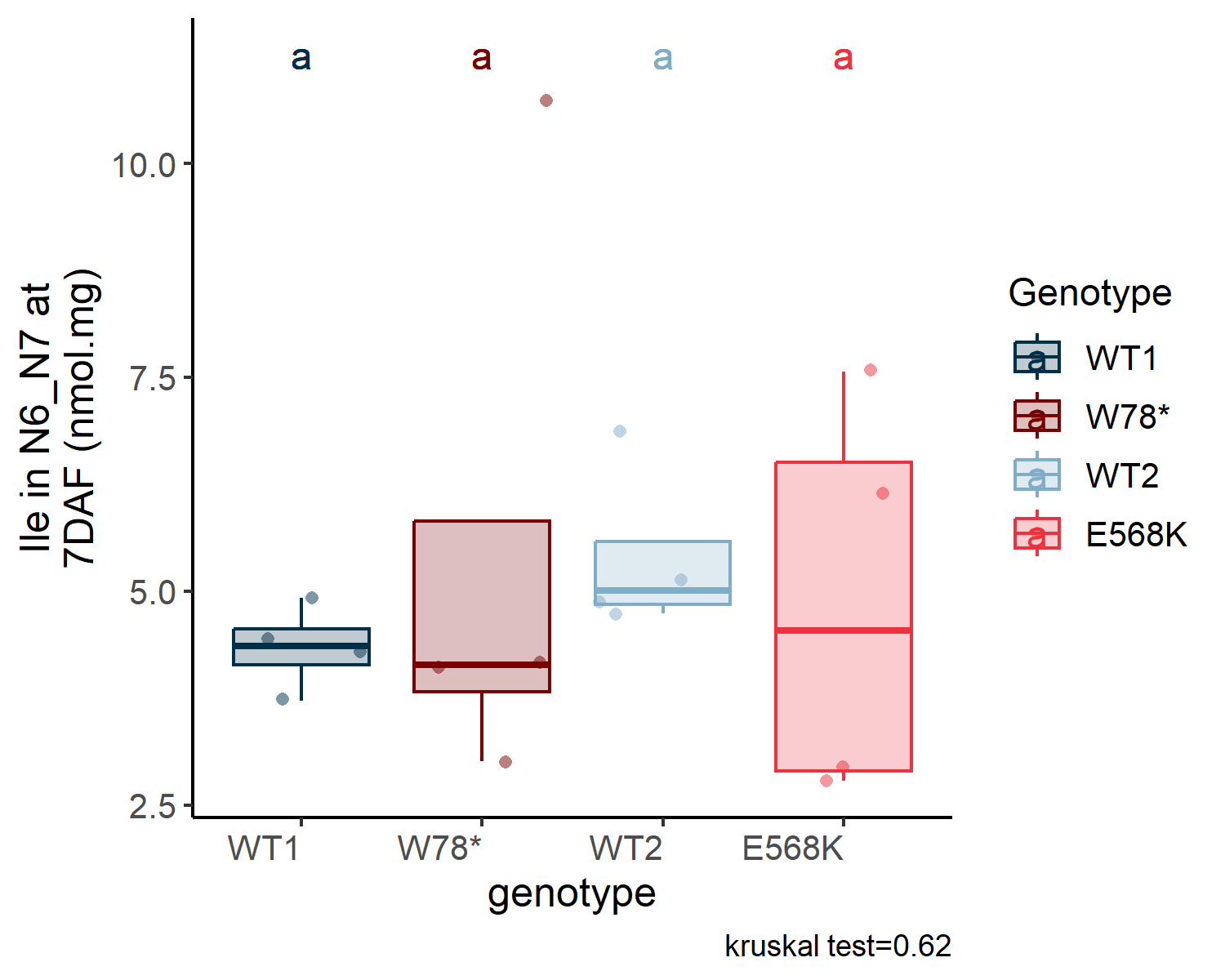
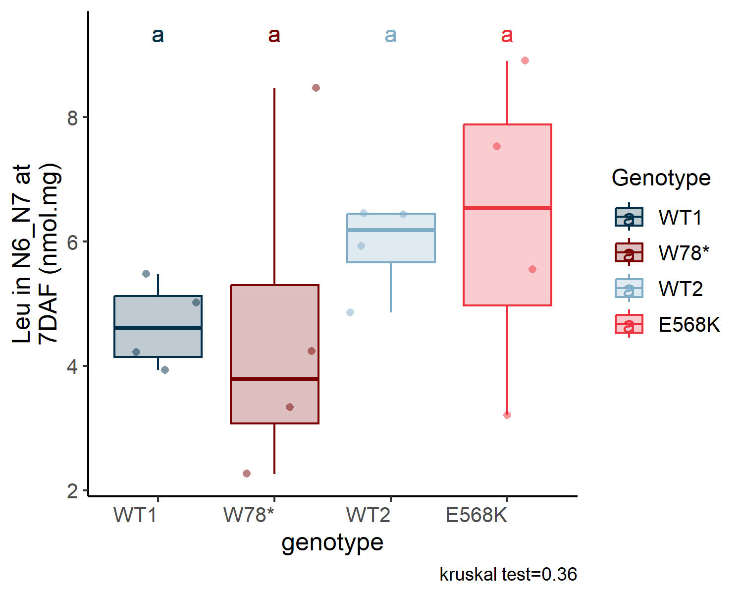
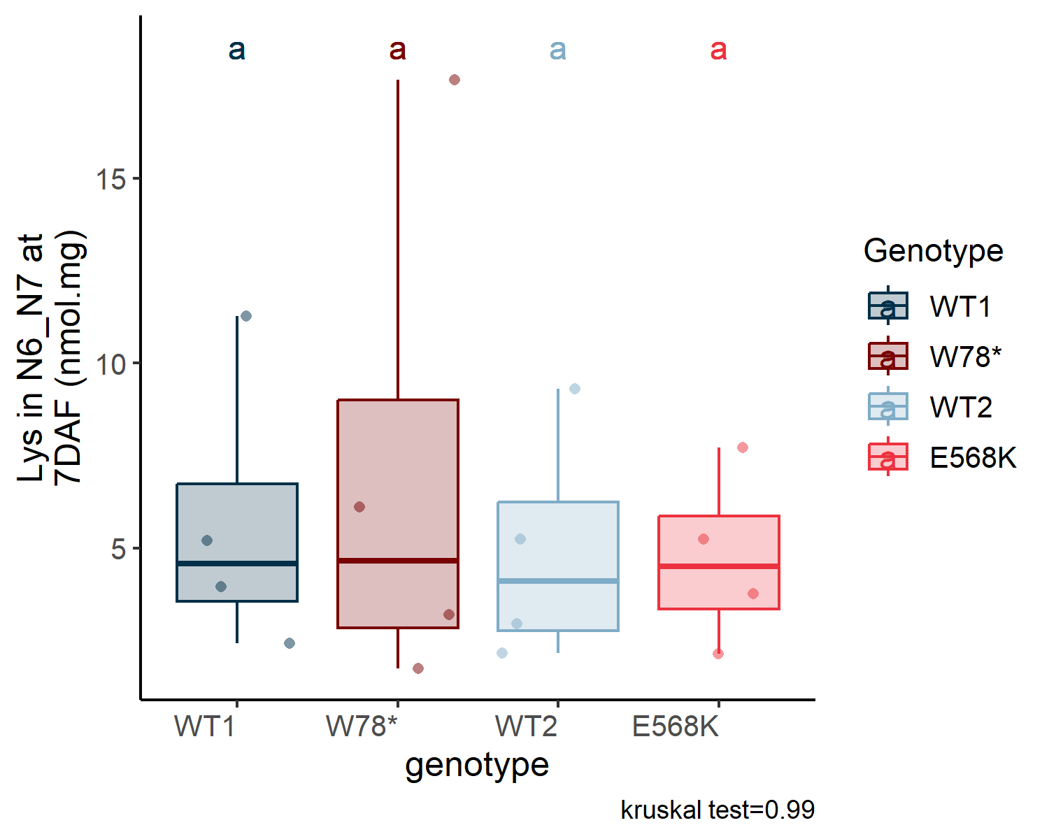
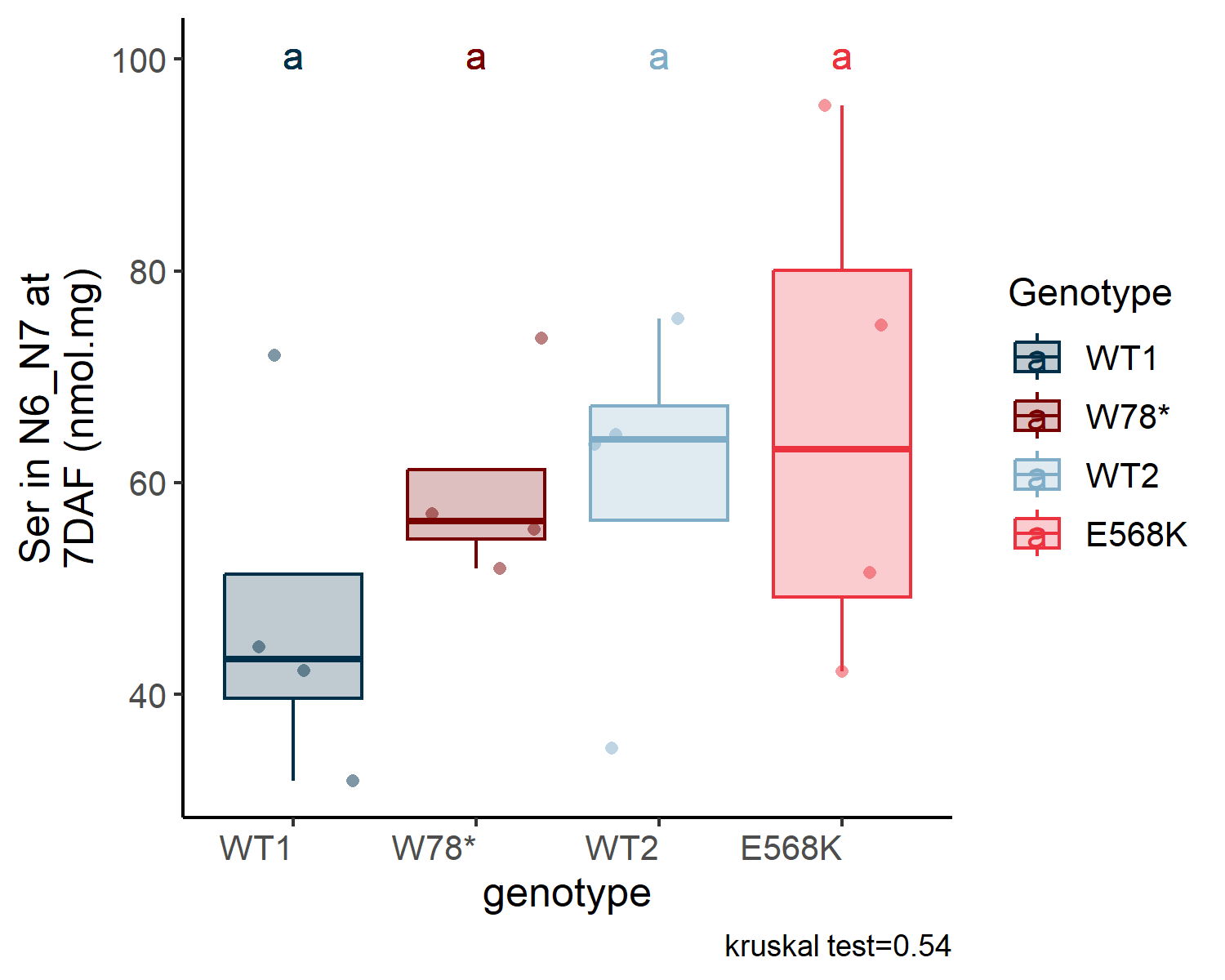
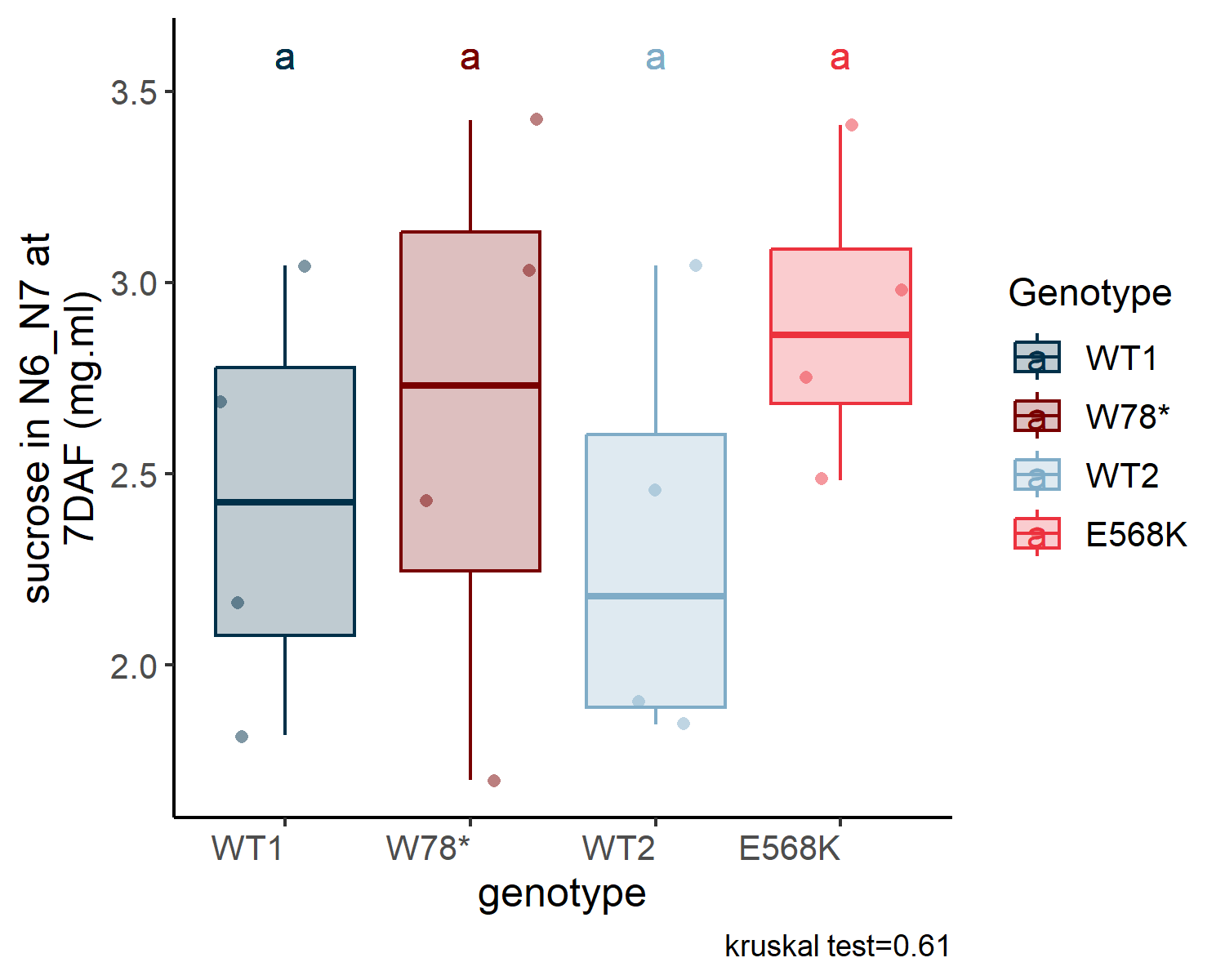
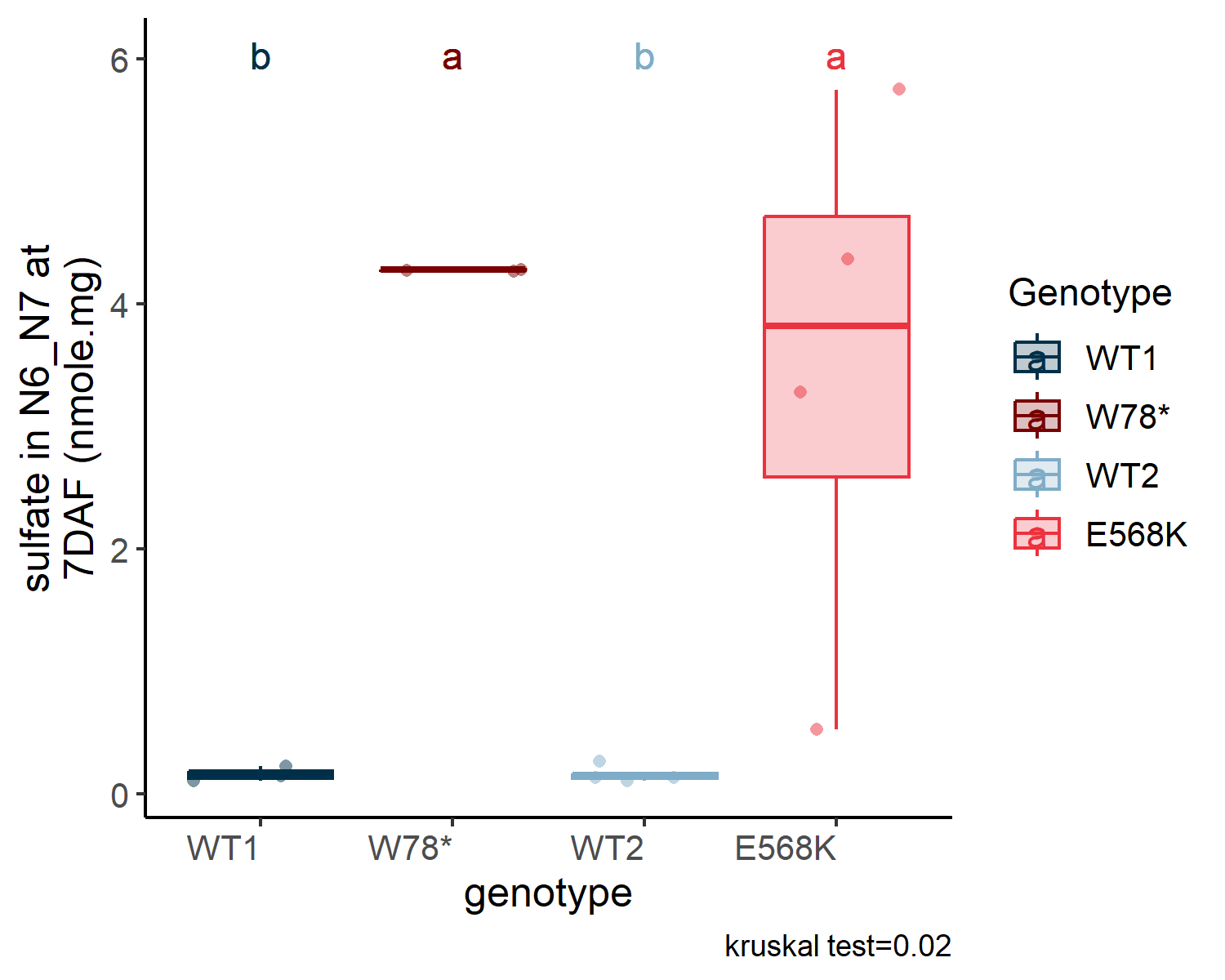
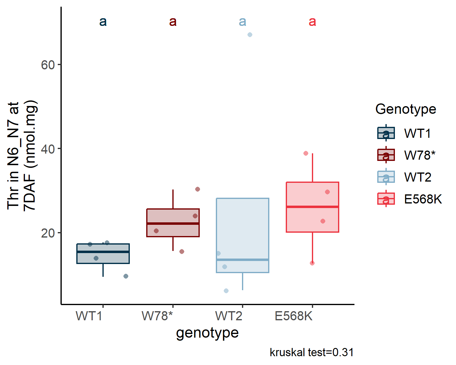
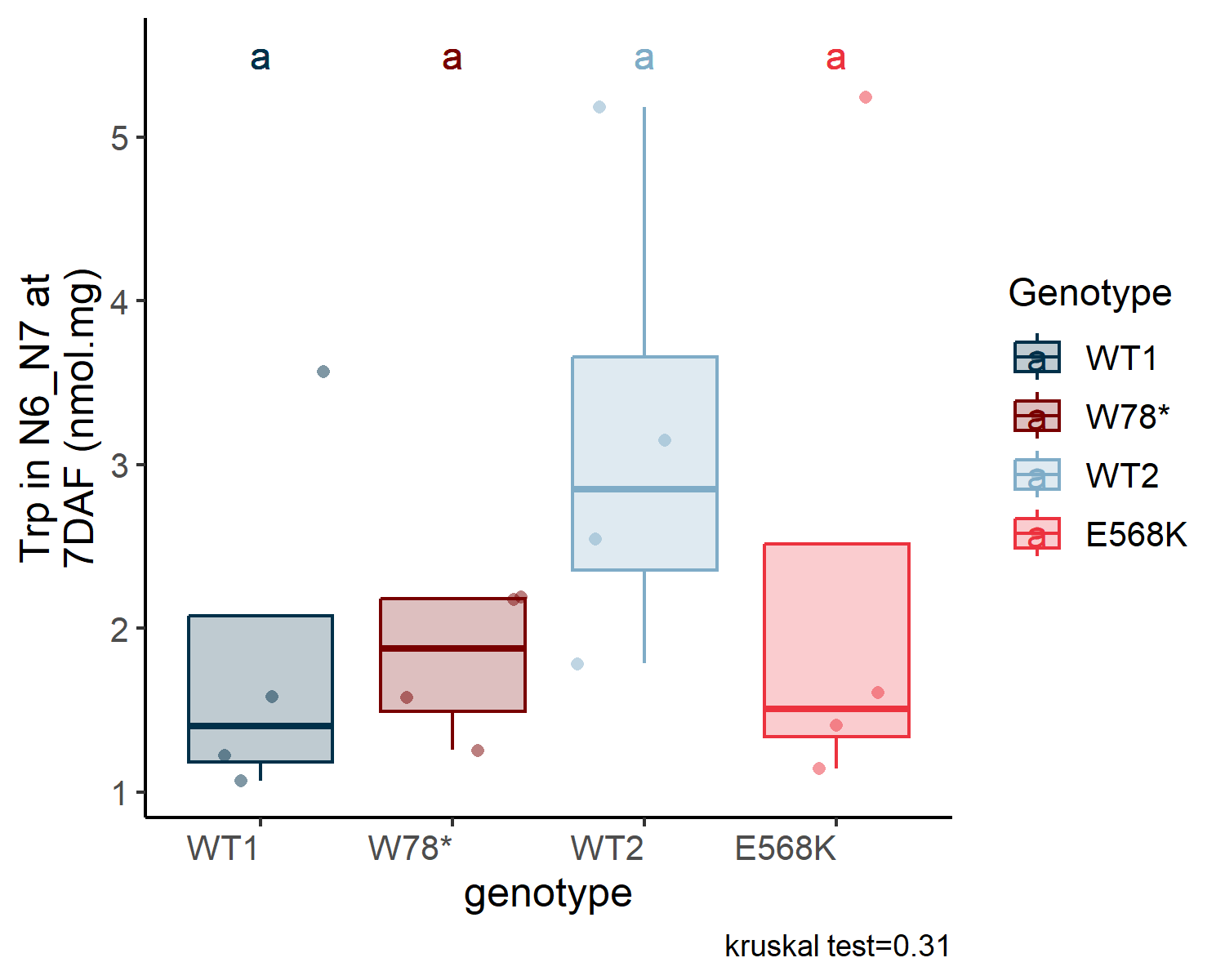
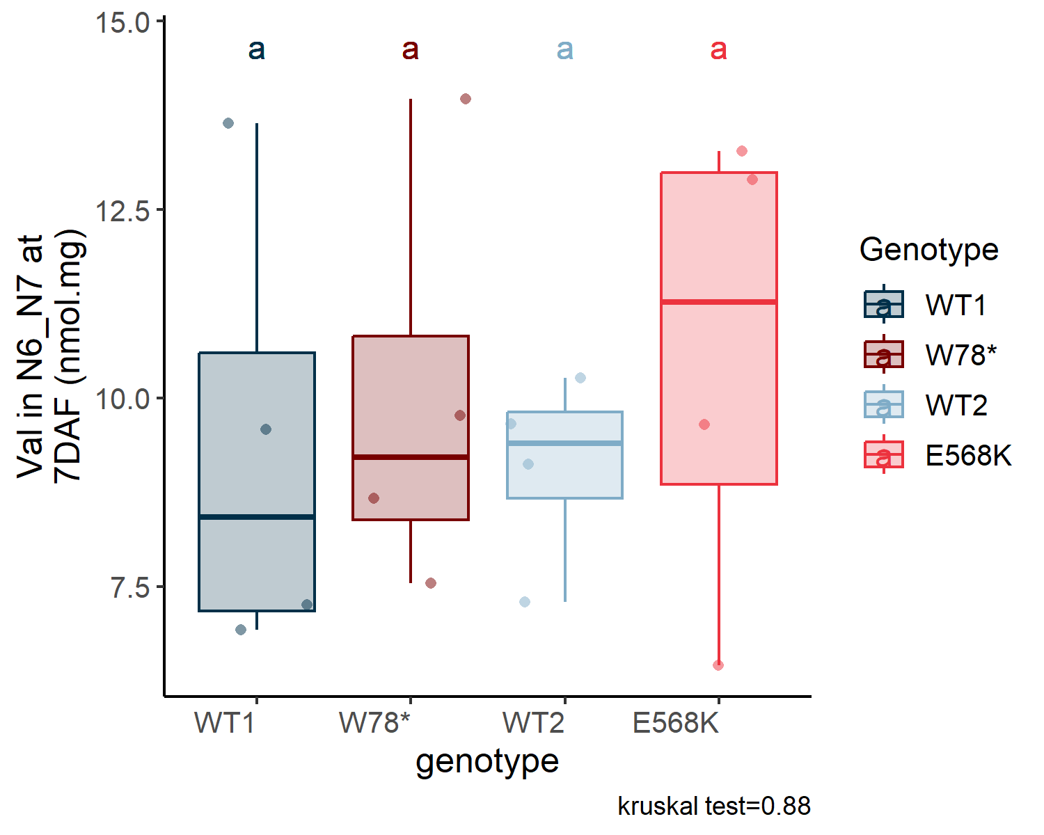
9  Metabolomic from IPS2

Code
#pkg
library(readxl)
library(tidyverse)
library(ggnewscale) # to have two scale_fill
library(ggh4x)
library(kableExtra)
library("FactoMineR")
library("factoextra")
library(patchwork)

# src
source(here::here("src/function/stat_function/stat_analysis_main.R")) # for make plot 
source(here::here("src/function/fig_export.R")) # This function saves a given plot (plot_x) as both a PDF and a high-resolution PNG file at specified dimensions.

# cosmetics
sulfate_pallet=read_excel(here::here("data/color_palette.xlsm")) %>%
      filter(set == "sulfure_condition") %>%
      dplyr::select(color, treatment) %>%
      pull(color) %>%
      setNames(read_excel(here::here("data/color_palette.xlsm")) %>%
                 filter(set == "sulfure_condition") %>%
                 pull(treatment)
               )

mutant_palette=read_excel(here::here("data/color_palette.xlsm")) %>%
      filter(set == "mutant") %>%
      dplyr::select(color, treatment) %>%
      pull(color) %>%
      setNames(read_excel(here::here("data/color_palette.xlsm")) %>%
                 filter(set == "mutant") %>%
                 pull(treatment)
               )

9.1 Material and methods

  • Data acquisition was performed on experiment 2.
    Data from IPS2 (Versailles)(received in July 2024), Experiment in Greenhouse 24 - September 2021 to November 2021

  • Data from Heidelberg (received in August 2024), Experiment in Greenhouse 24 - September 2021 to November 2021

Bonus:Here you’ll find the extraction and metabolome analysis methods for this experiment

9.1.1 Sulfate

Sulfate concentration was determined at the Metabolomic Core Technology Platform of Heidelberg University. Anions were extracted from ground plant tissues (20 mg freeze-dried powder) with 1.0 ml ultra-pure water for 45 min at 95°C. Samples were briefly cooled on ice and centrifuged at 4°C and 11 000x g for 15 min. 40 μL of the supernatant was transferred to plastic vials and diluted by adding 400 μL water. Anions, along with organic acids, were separated using an IonPac AS11-HC (2mm, ThermoScientific) column connected to an ICS-5000 system (ThermoScientific) and quantified by conductivity detection after cation suppression (ASRS-300 2mm, suppressor current 95-120 mA). Before separation, the column was heated to 30°C and equilibrated with five column volumes of solvent A (ultra-pure water) at a flow rate of 0.3 ml min-1. Separation of anions was achieved by increasing the concentration of solvent B (100 mM NaOH) in buffer A linearly as follows: 0-1 min. 4% B, 1-8 min. 4%-18% B, 8-9 min. 18-19% B, 9-15 min. 19%-30% B, 15-20 min. 30%-62% B, 20-20.1 min. 62%-80% B, 20.1-25 min. 80% B, 25-25.1 min. 80-4% B, and 25.1-35 min. 4% B. Data acquisition and quantification were performed with the Chromeleon 7 software (ThermoScientific).

9.1.2 Cysteine, GSH, OAS

Analyses were performed at the Metabolomic Core Technology Platform of Heidelberg University. Metabolites were extracted with 1 ml 0.1 M HCl using 20 mg dry weight of immature seeds and leaves (freeze-drying by lyophilization). Thiol and OAS were quantified after derivatization with monobromobimane (Calbiochem, EMD Chemicals) or AccQ-Tag reagent (Waters, USA), respectively. Thiols and OAS were derivatized and separated according to Wirtz et al., 2004 on an Acquity H-class system connected to the Acquity FLR-detector. Data acquisition and quantification were performed with the Empower Pro vs. 3.7.0 software suite (Waters, Germany).

9.1.3 Amino acids

The absolute quantification of amino acids and sugars was performed at the Platform Metabolism Metabolome (PMM, Institut des Sciences des Plantes de Paris-Saclay). Amino acid quantification was performed using OPA-HPLC (orthophtaladehyde-high performance liquid chromatography) profiling. Ground leaf samples (5 mg of freeze-dried powder) were resuspended in 1 ml of frozen (−20°C) water/acetonitrile/isopropanol (2:3:3) containing a-ABA (internal standard), ground, and centrifuged. Then, 150 μL of the supernatant/sample was dried for 4 h at 35°C in a Speed-Vac and stored at −80°C. Pre-column derivatization was performed in the injection loop by automated mixing of 10 μL sample and 10 μL OPA reagent, followed by a delay of 2 min prior to injection. The OPA reagent was made 48 h before first use by dissolving OPA at 10 mg ml−1 in 200 μL of methanol and adding 1.8 mL of 0.5 m sodium borate (pH 9.5) and 40 mL of 2-mercaptoethanol. The reagent was filtered into an autosampler vial and used for up to 3 days. An HPLC system (Agilent 1260 infinity) fitted with a fluorescence detector (Dual Absorbance, Agilent) was used. Compounds were detected at an excitation wavelength of 340 nm and an emission wavelength of 455 nm. Chromatographic separation was performed with a Symmetry C18 column (3.5 μm, 4.6 × 150 mm) by gradient elution at 40°C using buffer A (20% methanol, 80% sodium acetate, 1% tetrahydrofuran, pH 5.9) and buffer B (80% methanol, 20% sodium acetate, pH 5.9). The buffer flow rate was 0.7 ml min−1 and the total run time per injection was 42 min. The chromatography data were analyzed using the ChemStation software. Peak identity was confirmed by co-elution with authentic standards. Concentrations were calculated with calibration curves using the peak areas of compounds of interest.

9.1.4 Sugars

For quantification of sugars (fructose, glucose and sucrose) by HPLC, ground leaf samples (50 mg freeze-dried powder) were resuspended in 1 ml cold MilliQ water, stirred at 6°C for 40 min and centrifuged at 5°C (14 000g) for 15 min. The supernatants were heated at 100°C for 8 min, placed on ice for 30 min to allow denatured proteins to precipitate, then centrifuged at 5°C for 10 min. The supernatant (25 μL) was used for injection into a cation exchange column (SugarPack 6.5*300 mm, Waters). Elution was performed at 80°C in isocratic mode with milliQ water at a flow rate of 0.5 mL/min. Detection was performed with a refractometer. The chromatography data were analyzed using the ChemStation software with an Agilent 1260 infinity HPLC system. Peak identity was confirmed by co-elution with authentic standards. Concentrations were calculated with calibration curves using the peak areas of compounds of interest.

9.2 Data importation

Code
# amino acids
df_hplc_AA = 
  read.table(here::here("data/metabolomic/HPLC_AA_Raw_data.txt"), dec = ",", sep = "\t", header = TRUE, as.is = FALSE) %>% 
  dplyr::select(-c(Genotype_P_S, Num ,PSGF,Leaf)) %>% 
  separate(Plant_num_F, into = c("plant_num", "compartment"), sep = "_", convert = TRUE) %>% 
  dplyr::rename(sulfur_condition = S_condition, 
                genotype= Genotype, 
                stage = P) %>% 
  mutate(
    sulfur_condition = ifelse(sulfur_condition =="S+", "SS", "SD"),
    type_genotype = ifelse(genotype %in% c("WT1", "WT2"), "WT", "Mut"),
    type_variable = "AA",
    DAF = case_when(
      stage =="P1" ~ 7,
      stage =="P2" ~ 29,
      stage =="P3" ~ 37
    ),
    compartment = case_when(
      compartment =="FB" ~ "N4_N5",
      compartment =="FV" ~ "N6_N7",
      compartment =="FR" ~ "N9_N10"
    ),
    unit = "nmol.mg"
         ) %>% 
  pivot_longer(cols = c(Asp, Glu, Ser, Gln, Gly, Thr, Bala, Ala, GABA, Trp, Met, Val, Phe, Ile, Leu, Lys, Asn, hser), 
               names_to = "variable",
               values_to = "value") %>%
  mutate(sulfur_condition= fct_relevel(sulfur_condition, "SS", "SD"),
         genotype = fct_relevel(genotype, "WT1", "W78*", "WT2", "E568K"),
         compartment = fct_relevel(compartment, "N4_N5", "N6_N7","N9_N10"),
         type_genotype = fct_relevel(type_genotype, "WT", "Mut")
         )
  
# sugar
df_hplc_sugar = 
  read.table(here::here("data/metabolomic/HPLC_Sugar_Raw_data.txt"), dec = ",", sep = "\t", header = TRUE, as.is = FALSE) %>% 
  separate(Sample, into = c("plant_num", "compartment"), sep = "(?<=\\d)(?=[a-z])", convert = TRUE) %>% 
  separate(Genotype_P_S, into = c("genotype", "stage", "sulfur_condition"), sep = "_", convert = TRUE) %>%
  dplyr::rename(fructose = Fructose,
                glucose = Glucose,
                sucrose = Sucrose) %>% 
  mutate(
    sulfur_condition = ifelse(sulfur_condition =="S+", "SS", "SD"),
    type_genotype = ifelse(genotype %in% c("WT1", "WT2"), "WT", "Mut"),
    type_variable = "sugar",
    DAF = case_when(
      stage =="P1" ~ 7,
      stage =="P2" ~ 29,
      stage =="P3" ~ 37
    ),
    compartment = case_when(
      compartment =="fb" ~ "N4_N5",
      compartment =="fv" ~ "N6_N7",
      compartment =="fr" ~ "N9_N10"
    ),
    unit = "mg.ml"
         ) %>% 
  pivot_longer(cols = c(fructose, glucose, sucrose), 
               names_to = "variable",
               values_to = "value") %>%
  mutate(sulfur_condition= fct_relevel(sulfur_condition, "SS", "SD"),
         genotype = fct_relevel(genotype, "WT1", "W78*", "WT2", "E568K"),
         compartment = fct_relevel(compartment, "N4_N5", "N6_N7","N9_N10"),
         type_genotype = fct_relevel(type_genotype, "WT", "Mut")
         )

# sulfate cys GSH OAS
df_hplc_heidelberg_metabolite = 
  read.table(here::here("data/metabolomic/HPLC_Cysteine_OAS_GSH_Raw_data.txt"), dec = ",", sep = "\t", header = TRUE, as.is = FALSE) %>% 
  dplyr::select(-c(Weight_mg, ID, Name)) %>% 
  dplyr::rename(plant_num = Plant.num,
                sulfur_condition = Condition, 
                genotype= Genotype, 
                stage = Stage,
                compartment = Leaf,
                Cys = Cys_pmol.mg, 
                GSH = GSH_pmol.mg,
                OAS = OAS_pmol.mg) %>% 
  mutate(
    sulfur_condition = ifelse(sulfur_condition =="S+", "SS", "SD"),
    type_genotype = ifelse(genotype %in% c("WT1", "WT2"), "WT", "Mut"),
    type_variable = "other_metabolite",
    DAF = case_when(
      stage =="P1" ~ 7,
      stage =="P2" ~ 29,
      stage =="P3" ~ 37
    ),
    compartment = case_when(
      compartment =="FB" ~ "N4_N5",
      compartment =="FV" ~ "N6_N7",
      compartment =="FR" ~ "N9_N10"
    ),
    unit = "pmol.mg"
         ) %>% 
  pivot_longer(cols = c(Cys, GSH, OAS), 
               names_to = "variable",
               values_to = "value") %>% 
  mutate(sulfur_condition= fct_relevel(sulfur_condition, "SS", "SD"),
         genotype = fct_relevel(genotype, "WT1", "W78*", "WT2", "E568K"),
         compartment = fct_relevel(compartment, "N4_N5", "N6_N7"),
         type_genotype = fct_relevel(type_genotype, "WT", "Mut")
         )

# ions from Heidelberg
df_hplc_heidelberg_ion = 
  read.table(here::here("data/metabolomic/HPLC_sulfate_citrate_phosphate_Raw_data.txt"), dec = ",", sep = "\t", header = TRUE, as.is = FALSE) %>% 
  dplyr::select(-c(Weight_mg, ID, Name,Citrate_nmole.25µL, Phosphate_nmole.25µL, Sulfate_nmole.25µL)) %>% 
  dplyr::rename(plant_num = Plant.num,
                sulfur_condition = Condition, 
                genotype= Genotype, 
                stage = Stage,
                compartment = Leaf,
                citrate = Citrate_nmole.mg.FW, 
                phosphate = Phosphate_nmole.mg.FW,
                sulfate = Sulfate_nmole.mg.FW,
                ) %>% 
  mutate(
    sulfur_condition = ifelse(sulfur_condition =="S+", "SS", "SD"),
    type_genotype = ifelse(genotype %in% c("WT1", "WT2"), "WT", "Mut"),
    type_variable = "ion",
    DAF = case_when(
      stage =="P1" ~ 7,
      stage =="P2" ~ 29,
      stage =="P3" ~ 37
    ),
    compartment = case_when(
      compartment =="FB" ~ "N4_N5",
      compartment =="FV" ~ "N6_N7",
      compartment =="FR" ~ "N9_N10"
    ),
    unit = "nmole.mg"
         ) %>% 
  pivot_longer(cols = c(citrate, phosphate, sulfate), 
               names_to = "variable",
               values_to = "value") %>% 
  mutate(sulfur_condition= fct_relevel(sulfur_condition, "SS", "SD"),
         genotype = fct_relevel(genotype, "WT1", "W78*", "WT2", "E568K"),
         compartment = fct_relevel(compartment, "N4_N5", "N6_N7"),
         type_genotype = fct_relevel(type_genotype, "WT", "Mut")
         )

# colnames(df_hplc_AA)
# colnames(df_hplc_sugar)
# colnames(df_hplc_heidelberg_metabolite)
# colnames(df_hplc_heidelberg_ion)

df_metabolite_global = bind_rows(df_hplc_AA, df_hplc_sugar, df_hplc_heidelberg_metabolite,df_hplc_heidelberg_ion) %>% 
  mutate(condition = paste0(genotype, "_", sulfur_condition)) %>% 
  mutate(variable = if_else(str_detect(variable, "^[a-z\\s]+$"), 
                                 str_to_title(variable), 
                                 variable)) # uppercase letter only if all text is lowercase. 

# export data
write_csv(df_metabolite_global, here::here("data/metabolomic/output/df_metabolite_global.csv"))

9.3 Analysis summary table

Code
read_csv(here::here("data/metabolomic/output/df_metabolite_global.csv"), show_col_types = FALSE) %>% 
  mutate(plant_num = paste(sep = "_", plant_num, condition)) %>% 
  mutate(sulfur_condition= fct_relevel(sulfur_condition, "SS", "SD"),
         genotype = fct_relevel(genotype, "WT1", "W78*", "WT2", "E568K"),
         compartment = fct_relevel(compartment, "N4_N5", "N6_N7"),
         type_genotype = fct_relevel(type_genotype, "WT", "Mut")
         ) %>% 
  dplyr::group_by(condition, compartment, DAF, variable) %>% 
  dplyr::summarise(N=n(),.groups="drop") %>% 
  pivot_wider(names_from = variable, values_from = N) %>% 
  arrange(DAF, compartment) %>% 
  kbl(caption = "Data measure in metabolomic for the different metabolite, condition, compartment and DAF",digits = 2) %>% 
kable_paper(full_width = F) 
Code
type_metabo<-read_csv(here::here("data/metabolomic/output/df_metabolite_global.csv"), show_col_types = FALSE) %>% 
  dplyr::select(type_variable, variable) %>% 
  unique()

read_csv(here::here("data/metabolomic/output/df_metabolite_global.csv"), show_col_types = FALSE) %>% 
  dplyr::select(compartment, DAF, variable, condition) %>%
  mutate(DAF_compartment_condition = paste0("DAF:", DAF," ",compartment, " ", condition)
         #DAF_compartment = fct_relevel(DAF_compartment, "DAF:7 N6_N7", "DAF:29 N6_N7", "DAF:29 N9_N10", "DAF:37 N4_N5", "DAF:37 N6_N7", "DAF:37 N9_N10")) %>% 
  ) %>% 
  dplyr::group_by(DAF_compartment_condition, variable) %>% 
  dplyr::summarise(N=n(), .groups = "drop") %>% 
  ungroup() %>% 
  arrange(variable) %>% 
  left_join(.,type_metabo, by="variable") %>% 
  dplyr::group_by(type_variable,DAF_compartment_condition) %>%
  dplyr::summarize(compound_list =  paste(variable, collapse = ", "), .groups = 'drop') %>% 
  pivot_wider(names_from = DAF_compartment_condition, values_from = compound_list) %>% 
  dplyr::rename(`Type of variable` = type_variable) %>% 
  kable(format = "html", booktabs = TRUE) %>%
  kable_styling(bootstrap_options = c("striped", "hover", "condensed", "responsive")) %>%
  row_spec(0, extra_css = "vertical-align: middle;")
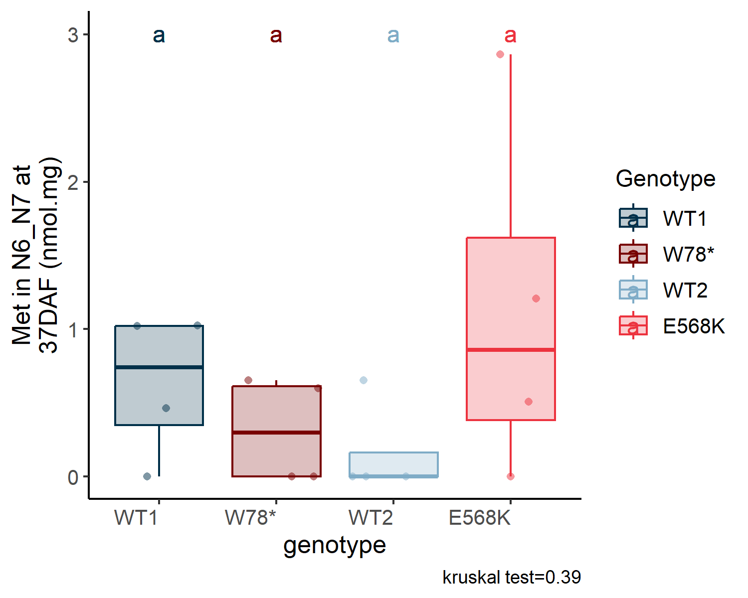
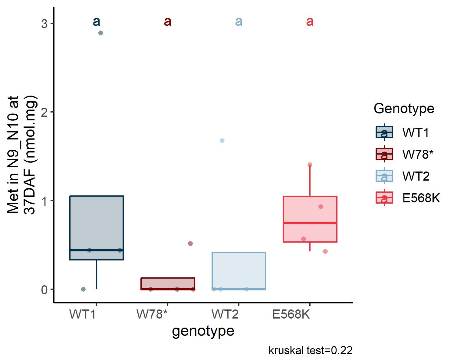
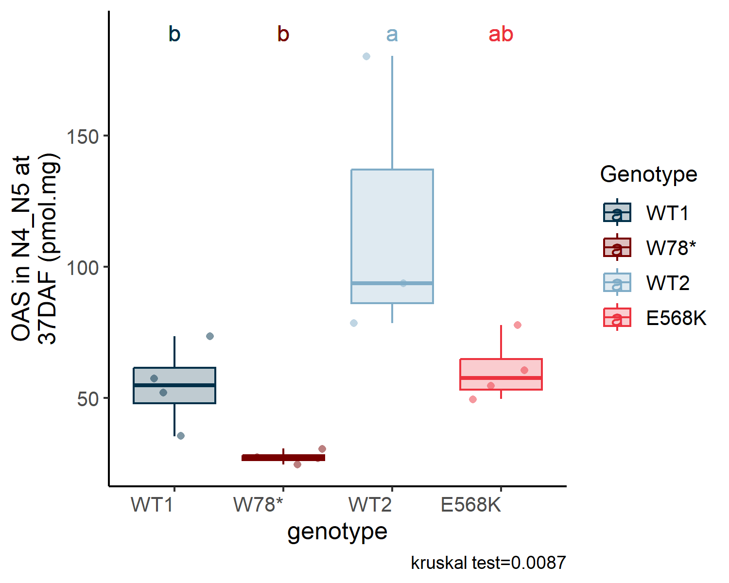
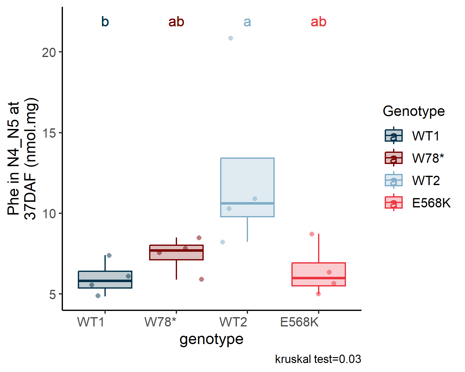
Type of variable DAF:29 N6_N7 E568K_SD DAF:29 N6_N7 W78*_SD DAF:29 N6_N7 WT1_SD DAF:29 N6_N7 WT1_SS DAF:29 N6_N7 WT2_SD DAF:29 N6_N7 WT2_SS DAF:29 N9_N10 E568K_SD DAF:29 N9_N10 W78*_SD DAF:29 N9_N10 WT1_SD DAF:29 N9_N10 WT1_SS DAF:29 N9_N10 WT2_SD DAF:29 N9_N10 WT2_SS DAF:37 N4_N5 E568K_SD DAF:37 N4_N5 W78*_SD DAF:37 N4_N5 WT1_SD DAF:37 N4_N5 WT1_SS DAF:37 N4_N5 WT2_SD DAF:37 N4_N5 WT2_SS DAF:37 N6_N7 E568K_SD DAF:37 N6_N7 W78*_SD DAF:37 N6_N7 WT1_SD DAF:37 N6_N7 WT1_SS DAF:37 N6_N7 WT2_SD DAF:37 N6_N7 WT2_SS DAF:37 N9_N10 E568K_SD DAF:37 N9_N10 W78*_SD DAF:37 N9_N10 WT1_SD DAF:37 N9_N10 WT1_SS DAF:37 N9_N10 WT2_SD DAF:37 N9_N10 WT2_SS DAF:7 N6_N7 E568K_SD DAF:7 N6_N7 W78*_SD DAF:7 N6_N7 WT1_SD DAF:7 N6_N7 WT1_SS DAF:7 N6_N7 WT2_SD DAF:7 N6_N7 WT2_SS
AA Ala, Asn, Asp, Bala, GABA, Gln, Glu, Gly, Hser, Ile, Leu, Lys, Met, Phe, Ser, Thr, Trp, Val Ala, Asn, Asp, Bala, GABA, Gln, Glu, Gly, Hser, Ile, Leu, Lys, Met, Phe, Ser, Thr, Trp, Val Ala, Asn, Asp, Bala, GABA, Gln, Glu, Gly, Hser, Ile, Leu, Lys, Met, Phe, Ser, Thr, Trp, Val Ala, Asn, Asp, Bala, GABA, Gln, Glu, Gly, Hser, Ile, Leu, Lys, Met, Phe, Ser, Thr, Trp, Val Ala, Asn, Asp, Bala, GABA, Gln, Glu, Gly, Hser, Ile, Leu, Lys, Met, Phe, Ser, Thr, Trp, Val Ala, Asn, Asp, Bala, GABA, Gln, Glu, Gly, Hser, Ile, Leu, Lys, Met, Phe, Ser, Thr, Trp, Val Ala, Asn, Asp, Bala, GABA, Gln, Glu, Gly, Hser, Ile, Leu, Lys, Met, Phe, Ser, Thr, Trp, Val Ala, Asn, Asp, Bala, GABA, Gln, Glu, Gly, Hser, Ile, Leu, Lys, Met, Phe, Ser, Thr, Trp, Val Ala, Asn, Asp, Bala, GABA, Gln, Glu, Gly, Hser, Ile, Leu, Lys, Met, Phe, Ser, Thr, Trp, Val Ala, Asn, Asp, Bala, GABA, Gln, Glu, Gly, Hser, Ile, Leu, Lys, Met, Phe, Ser, Thr, Trp, Val Ala, Asn, Asp, Bala, GABA, Gln, Glu, Gly, Hser, Ile, Leu, Lys, Met, Phe, Ser, Thr, Trp, Val Ala, Asn, Asp, Bala, GABA, Gln, Glu, Gly, Hser, Ile, Leu, Lys, Met, Phe, Ser, Thr, Trp, Val Ala, Asn, Asp, Bala, GABA, Gln, Glu, Gly, Hser, Ile, Leu, Lys, Met, Phe, Ser, Thr, Trp, Val Ala, Asn, Asp, Bala, GABA, Gln, Glu, Gly, Hser, Ile, Leu, Lys, Met, Phe, Ser, Thr, Trp, Val Ala, Asn, Asp, Bala, GABA, Gln, Glu, Gly, Hser, Ile, Leu, Lys, Met, Phe, Ser, Thr, Trp, Val Ala, Asn, Asp, Bala, GABA, Gln, Glu, Gly, Hser, Ile, Leu, Lys, Met, Phe, Ser, Thr, Trp, Val Ala, Asn, Asp, Bala, GABA, Gln, Glu, Gly, Hser, Ile, Leu, Lys, Met, Phe, Ser, Thr, Trp, Val Ala, Asn, Asp, Bala, GABA, Gln, Glu, Gly, Hser, Ile, Leu, Lys, Met, Phe, Ser, Thr, Trp, Val Ala, Asn, Asp, Bala, GABA, Gln, Glu, Gly, Hser, Ile, Leu, Lys, Met, Phe, Ser, Thr, Trp, Val Ala, Asn, Asp, Bala, GABA, Gln, Glu, Gly, Hser, Ile, Leu, Lys, Met, Phe, Ser, Thr, Trp, Val Ala, Asn, Asp, Bala, GABA, Gln, Glu, Gly, Hser, Ile, Leu, Lys, Met, Phe, Ser, Thr, Trp, Val Ala, Asn, Asp, Bala, GABA, Gln, Glu, Gly, Hser, Ile, Leu, Lys, Met, Phe, Ser, Thr, Trp, Val Ala, Asn, Asp, Bala, GABA, Gln, Glu, Gly, Hser, Ile, Leu, Lys, Met, Phe, Ser, Thr, Trp, Val Ala, Asn, Asp, Bala, GABA, Gln, Glu, Gly, Hser, Ile, Leu, Lys, Met, Phe, Ser, Thr, Trp, Val Ala, Asn, Asp, Bala, GABA, Gln, Glu, Gly, Hser, Ile, Leu, Lys, Met, Phe, Ser, Thr, Trp, Val Ala, Asn, Asp, Bala, GABA, Gln, Glu, Gly, Hser, Ile, Leu, Lys, Met, Phe, Ser, Thr, Trp, Val Ala, Asn, Asp, Bala, GABA, Gln, Glu, Gly, Hser, Ile, Leu, Lys, Met, Phe, Ser, Thr, Trp, Val Ala, Asn, Asp, Bala, GABA, Gln, Glu, Gly, Hser, Ile, Leu, Lys, Met, Phe, Ser, Thr, Trp, Val Ala, Asn, Asp, Bala, GABA, Gln, Glu, Gly, Hser, Ile, Leu, Lys, Met, Phe, Ser, Thr, Trp, Val Ala, Asn, Asp, Bala, GABA, Gln, Glu, Gly, Hser, Ile, Leu, Lys, Met, Phe, Ser, Thr, Trp, Val Ala, Asn, Asp, Bala, GABA, Gln, Glu, Gly, Hser, Ile, Leu, Lys, Met, Phe, Ser, Thr, Trp, Val Ala, Asn, Asp, Bala, GABA, Gln, Glu, Gly, Hser, Ile, Leu, Lys, Met, Phe, Ser, Thr, Trp, Val Ala, Asn, Asp, Bala, GABA, Gln, Glu, Gly, Hser, Ile, Leu, Lys, Met, Phe, Ser, Thr, Trp, Val Ala, Asn, Asp, Bala, GABA, Gln, Glu, Gly, Hser, Ile, Leu, Lys, Met, Phe, Ser, Thr, Trp, Val Ala, Asn, Asp, Bala, GABA, Gln, Glu, Gly, Hser, Ile, Leu, Lys, Met, Phe, Ser, Thr, Trp, Val Ala, Asn, Asp, Bala, GABA, Gln, Glu, Gly, Hser, Ile, Leu, Lys, Met, Phe, Ser, Thr, Trp, Val
ion Citrate, Phosphate, Sulfate Citrate, Phosphate, Sulfate Citrate, Phosphate, Sulfate NA Citrate, Phosphate, Sulfate Citrate, Phosphate, Sulfate NA NA NA NA NA NA Citrate, Phosphate, Sulfate Citrate, Phosphate, Sulfate Citrate, Phosphate, Sulfate Citrate, Phosphate, Sulfate Citrate, Phosphate, Sulfate Citrate, Phosphate, Sulfate NA NA Citrate, Phosphate, Sulfate NA NA NA NA NA NA NA NA NA Citrate, Phosphate, Sulfate Citrate, Phosphate, Sulfate Citrate, Phosphate, Sulfate Citrate, Phosphate, Sulfate Citrate, Phosphate, Sulfate Citrate, Phosphate, Sulfate
other_metabolite Cys, GSH, OAS Cys, GSH, OAS Cys, GSH, OAS NA Cys, GSH, OAS Cys, GSH, OAS NA NA NA NA NA NA Cys, GSH, OAS Cys, GSH, OAS Cys, GSH, OAS Cys, GSH, OAS Cys, GSH, OAS Cys, GSH, OAS NA NA Cys, GSH, OAS NA NA NA NA NA NA NA NA NA Cys, GSH, OAS Cys, GSH, OAS Cys, GSH, OAS Cys, GSH, OAS Cys, GSH, OAS Cys, GSH, OAS
sugar Fructose, Glucose, Sucrose Fructose, Glucose, Sucrose Fructose, Glucose, Sucrose Fructose, Glucose, Sucrose Fructose, Glucose, Sucrose Fructose, Glucose, Sucrose Fructose, Glucose, Sucrose Fructose, Glucose, Sucrose Fructose, Glucose, Sucrose Fructose, Glucose, Sucrose Fructose, Glucose, Sucrose Fructose, Glucose, Sucrose Fructose, Glucose, Sucrose Fructose, Glucose, Sucrose Fructose, Glucose, Sucrose Fructose, Glucose, Sucrose Fructose, Glucose, Sucrose Fructose, Glucose, Sucrose Fructose, Glucose, Sucrose Fructose, Glucose, Sucrose Fructose, Glucose, Sucrose Fructose, Glucose, Sucrose Fructose, Glucose, Sucrose Fructose, Glucose, Sucrose Fructose, Glucose, Sucrose Fructose, Glucose, Sucrose Fructose, Glucose, Sucrose Fructose, Glucose, Sucrose Fructose, Glucose, Sucrose Fructose, Glucose, Sucrose Fructose, Glucose, Sucrose Fructose, Glucose, Sucrose Fructose, Glucose, Sucrose Fructose, Glucose, Sucrose Fructose, Glucose, Sucrose Fructose, Glucose, Sucrose

9.4 Analysis

Code
df_metabolite_global <- read_csv(here::here("data/metabolomic/output/df_metabolite_global.csv"), show_col_types = FALSE) %>% 
  mutate(plant_num = paste(sep = "_", plant_num, condition)) %>% 
  mutate(sulfur_condition= fct_relevel(sulfur_condition, "SS", "SD"),
         genotype = fct_relevel(genotype, "WT1", "W78*", "WT2", "E568K"),
         compartment = fct_relevel(compartment, "N4_N5", "N6_N7"),
         type_genotype = fct_relevel(type_genotype, "WT", "Mut")
         )

make_PCA_genotype <- function(df_info, norm = T){
  df <- df_info %>% select(-c("condition", "genotype", "sulfur_condition","type_genotype"))
  res_pca <- PCA(df, quali.sup = 1:4, graph = F)
  
  #fviz_eig(res_pca, addlabels = TRUE, ylim = c(0, 50))
  var <- get_pca_var(res_pca)
  PCA_indiv<-fviz_pca_ind(res_pca,
   #            geom.ind = "point", # Shows points only (not text)
               #pointshape = 20,pointsize = 2,
               col.ind = df_info %>% pull(genotype), # colorer by groups
               shape.ind   = df_info$genotype_simplify,  # Forme selon le génotype
               palett= c("#003049", "#780000", "#7FACC7", "#EC323E"),
               addEllipses = T, # Concentration ellipses
               legend.title = "Treatment", 
               ellipse.level = 0.95,
               ellipse.type = c("norm")
               
  )+ ggtitle(paste0("Visualizing Individual PCA by genotype for ",df_info$sulfur_condition[1], " at 37 DAF"))
  return(PCA_indiv)
}

# PCA
df_metabolite_global_select <- df_metabolite_global %>% 
  filter(compartment == "N4_N5",
         DAF == "37",
         sulfur_condition == "SD") %>% 
  dplyr::select(plant_num, condition,sulfur_condition, genotype,type_genotype, variable, value) %>% 
   pivot_wider(names_from = variable, values_from = value) %>%
  column_to_rownames("plant_num")

make_PCA_genotype(df_metabolite_global_select)
Code
df_metabolite_global <- read_csv(here::here("data/metabolomic/output/df_metabolite_global.csv"), show_col_types = FALSE) %>% 
  mutate(sulfur_condition= fct_relevel(sulfur_condition, "SS", "SD"),
         genotype = forcats::fct_relevel(genotype, "WT1", "W78*", "WT2", "E568K"),
         compartment = fct_relevel(compartment, "N4_N5", "N6_N7"),
         condition = paste(sep = "_", genotype, sulfur_condition), 
         condition = forcats::fct_relevel(condition, "WT1_SS", "WT1_SD",
                                          #"W78*_SS", 
                                          "W78*_SD", "WT2_SS", "WT2_SD", #"E568K_SS",
                                          "E568K_SD"),
         type_genotype = fct_relevel(type_genotype, "WT", "Mut")
         )

all_possibility <- df_metabolite_global %>%
  filter(sulfur_condition == "SD") %>%  
  distinct(DAF, variable, compartment)

plots <- list()

for (i in seq_len(nrow(all_possibility))) {
  
  DAF_i <- all_possibility$DAF[i]
  variable_i <- all_possibility$variable[i]
  compartment_i <- all_possibility$compartment[i]
 
  # Filtrage des données pour la combinaison courante
  df_select <- df_metabolite_global %>% 
    filter(
      sulfur_condition == "SD",
      DAF == DAF_i, 
      variable == variable_i,
      compartment == compartment_i
    ) %>% 
    drop_na(value) %>% 
    as.data.frame()
  
  # Si aucune donnée n'est disponible, on passe à la combinaison suivante
  if(nrow(df_select) == 0) {
    message("Aucune donnée pour: ", DAF_i, ", ", variable_i, ", ", compartment_i)
    next
  }
  
  # Définition de l'étiquette de l'axe des ordonnées
  ylab_i <-  paste0(variable_i, " in ", compartment_i, " at\n", DAF_i, "DAF (",df_select %>% 
  head(1) %>%
  pull(unit),")")
  
  # Essayer d'exécuter stat_analyse et capturer les erreurs éventuelles
  res <- tryCatch({
      stat_analyse(
        data = df_select,
        column_value = "value",
        category_variables = c("genotype"),
        grp_var = "",
        show_plot = TRUE,
        outlier_show = FALSE, 
        label_outlier = "plant_num",
        biologist_stats = TRUE,
        Ylab_i = ylab_i,
        control_conditions = "",
        strip_normale = FALSE,
        hex_pallet =  c("#003049", "#780000", "#7FACC7", "#EC323E")
      )
    },
    error = function(e) {
      message("Erreur pour: ", DAF_i, ", ", variable_i, ", ", compartment_i, " -> ", e$message)
      return(NULL)
    })
  
  # Si une erreur s'est produite, on passe à l'itération suivante
  if(is.null(res)) next
  
  # Extraction du plot et ajout des labels pour la légende
  p_plot <- res[["plot"]] + labs(color = "Genotype", fill = "Genotype")
  
  plot_name <- paste0("DAF",as.character(DAF_i), "_", variable_i,"_", compartment_i)
  
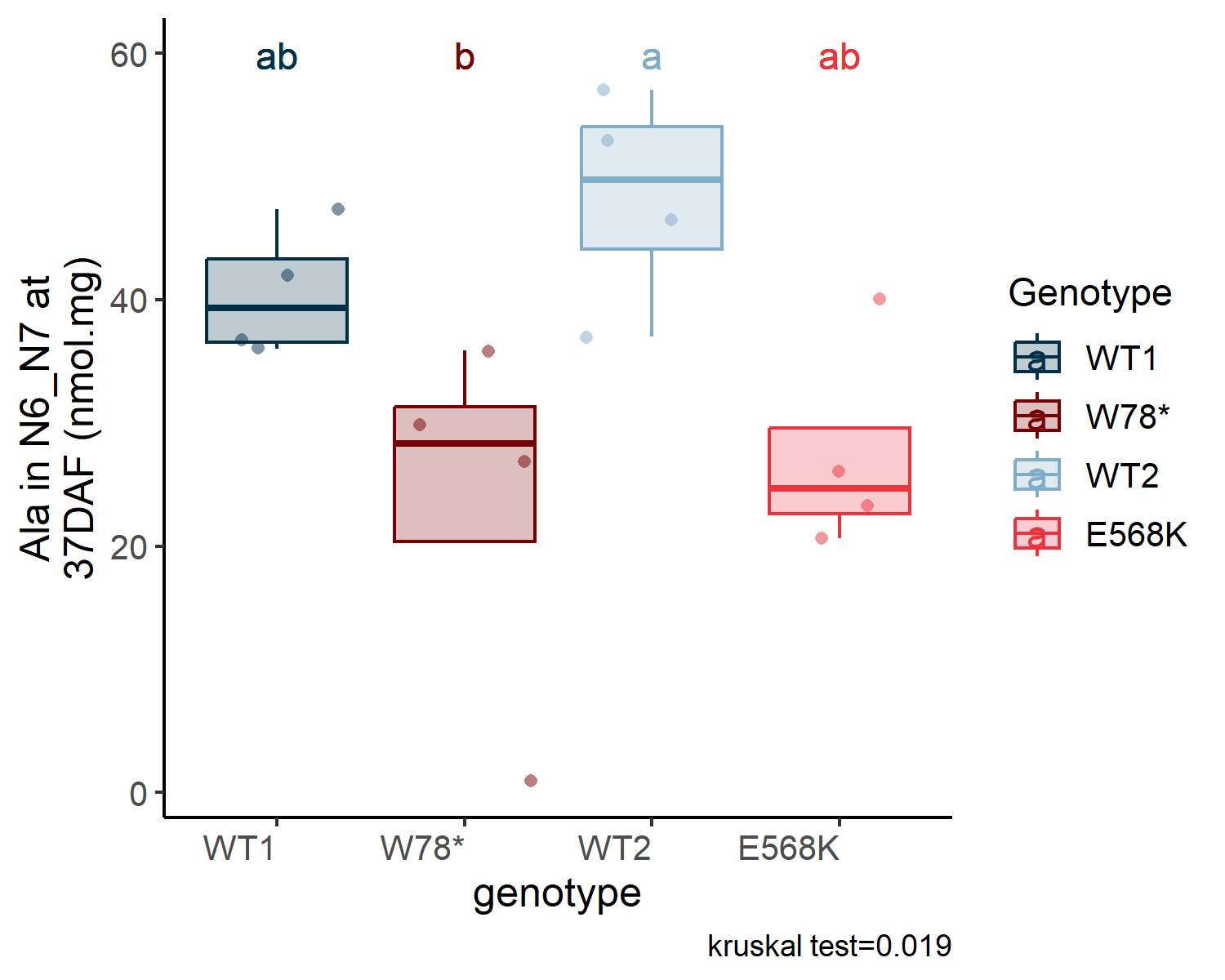
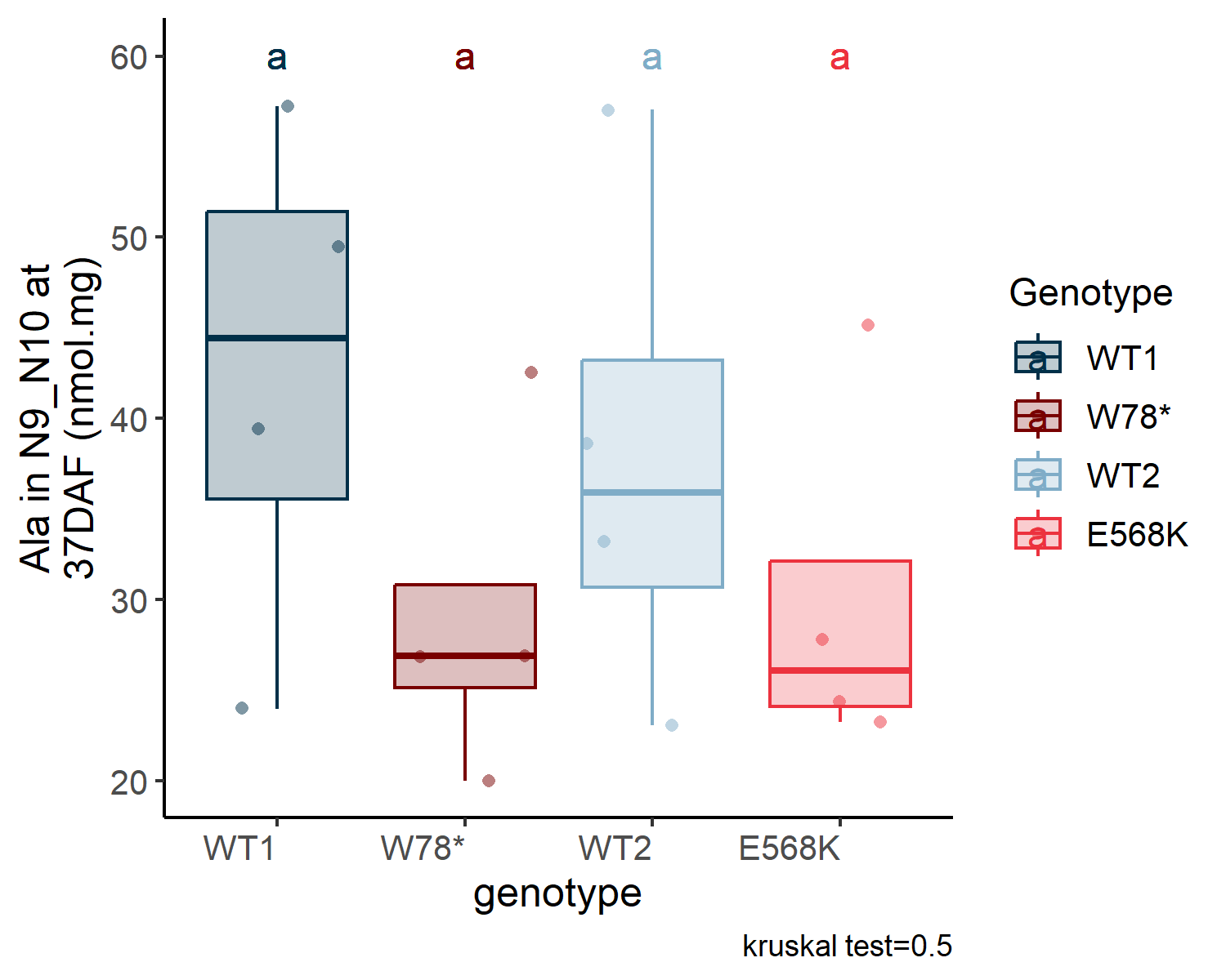
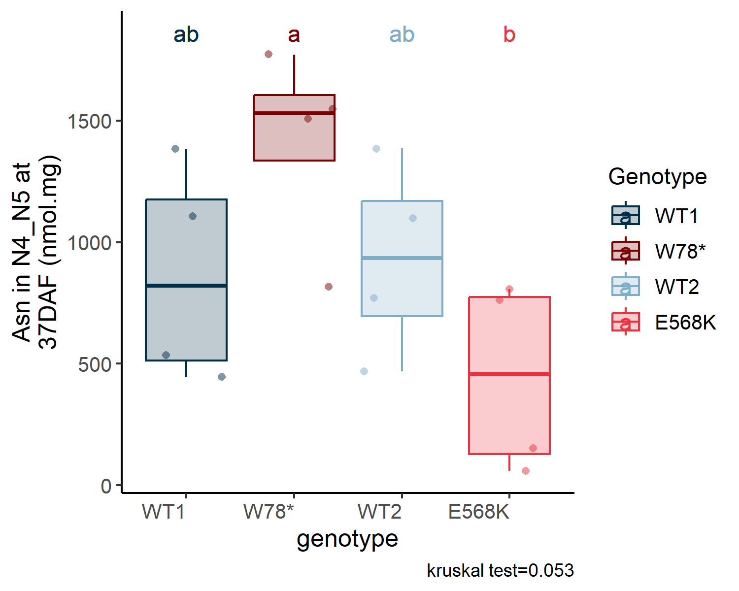
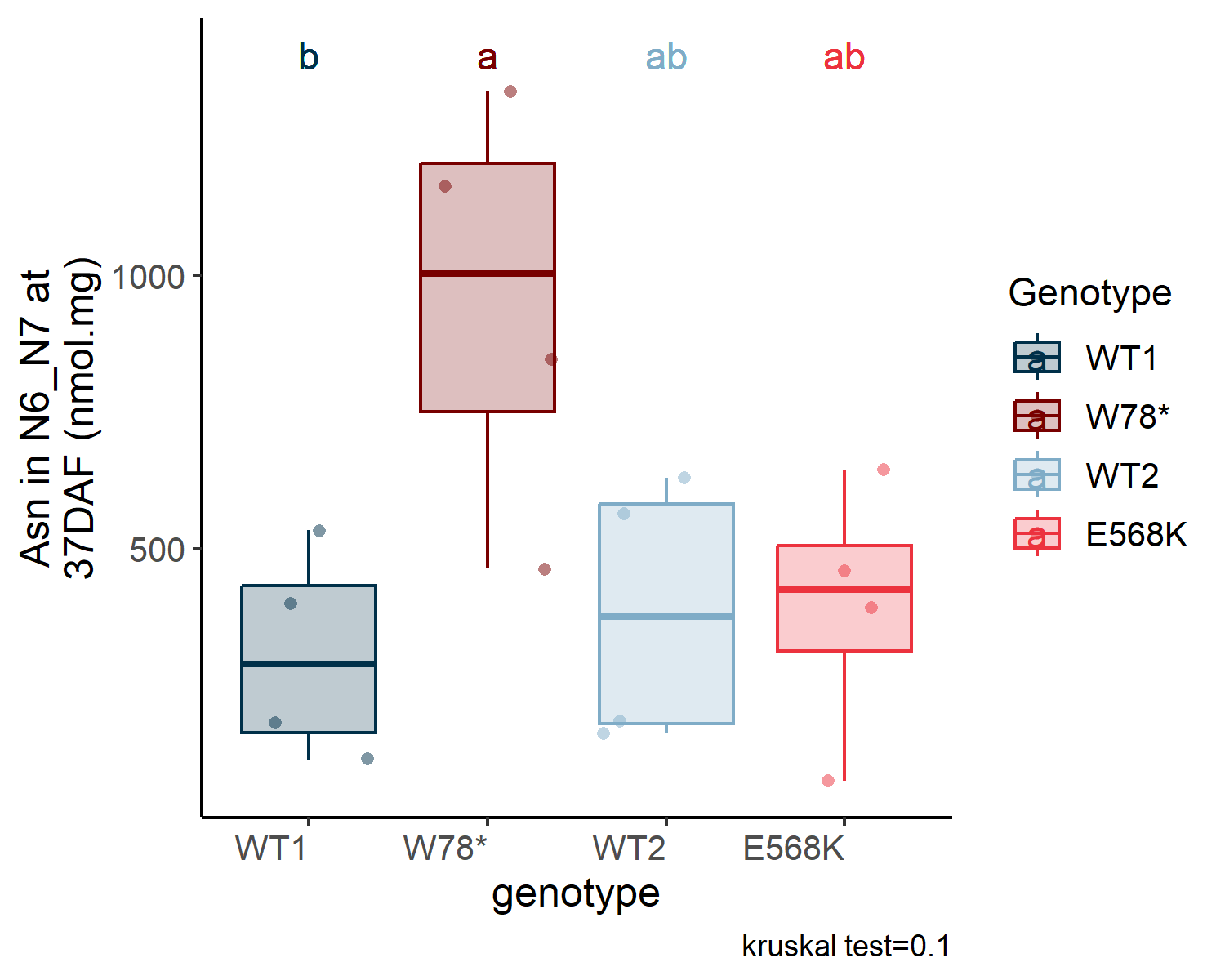
  fig_export(here::here(paste0("report/metabolomic/plot/SD_metabo/", plot_name)), p_plot, height_i = 4, width_i = 5, res_i = 300,format = "png")
  
  # Stockage du plot dans la liste avec un nom unique
  plots[[plot_name]] <- p_plot
}

# Assemblage de tous les plots avec patchwork
final_plot <- wrap_plots(plots, ncol = 8) +
  plot_layout(guides = "collect") +
  theme(legend.position = 'bottom')

# Affichage du plot final
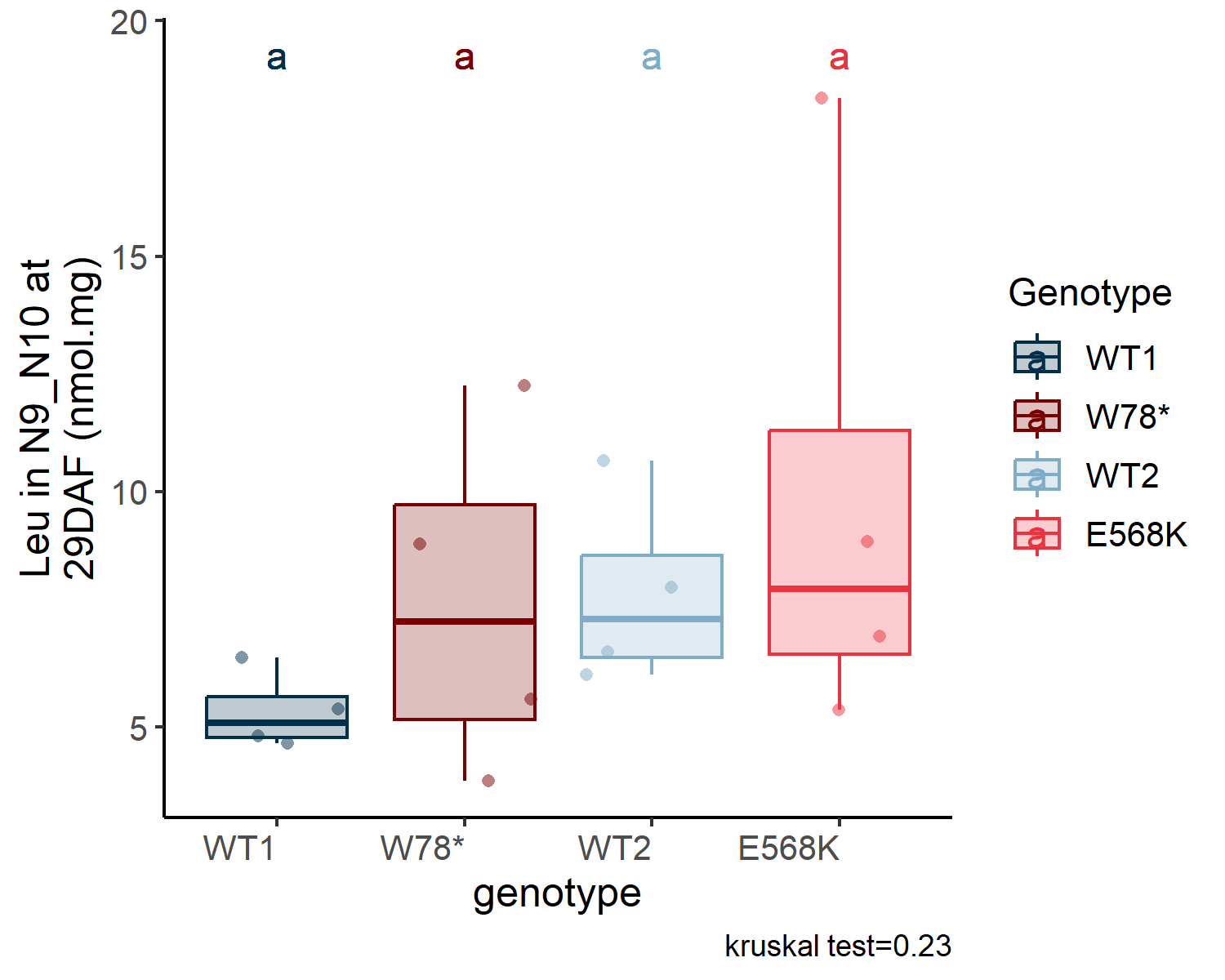
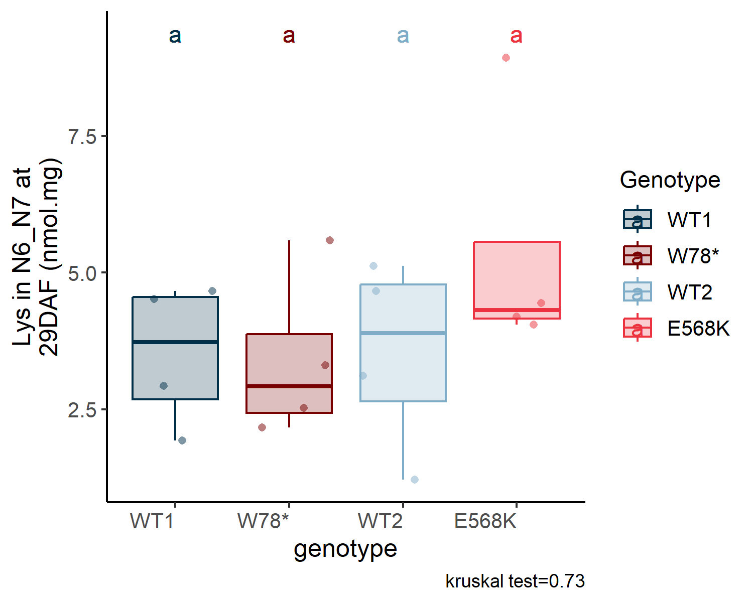
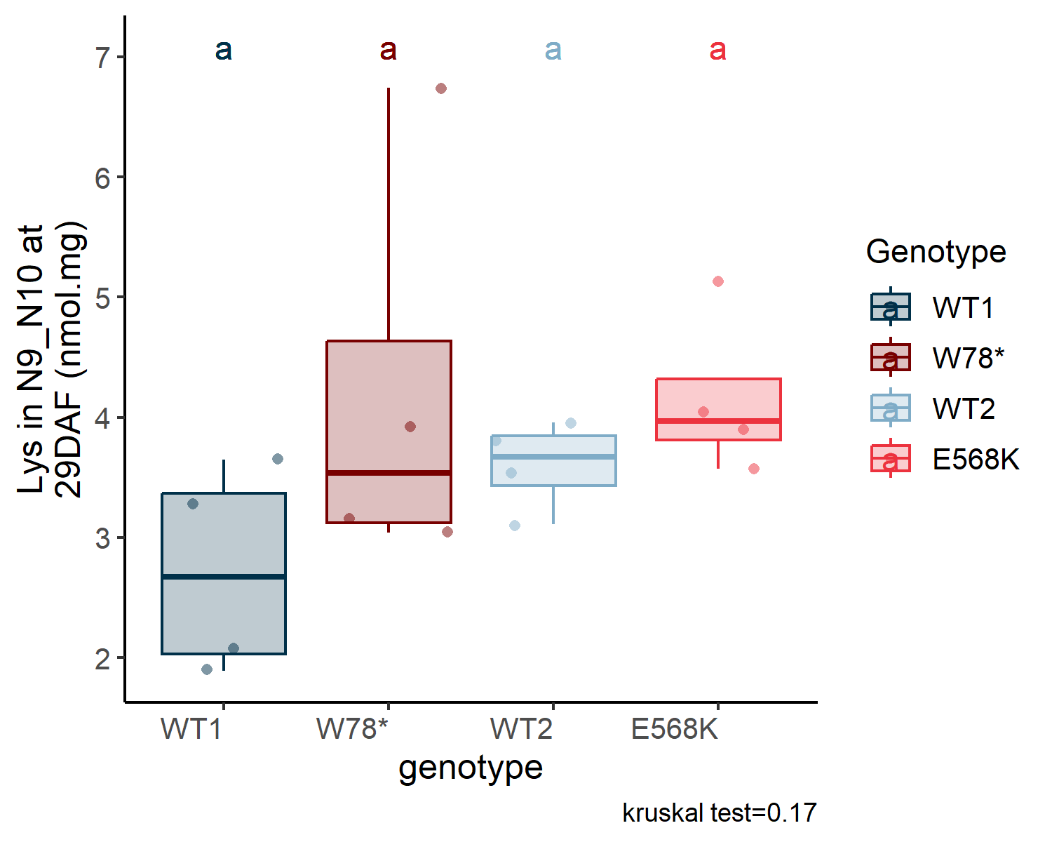
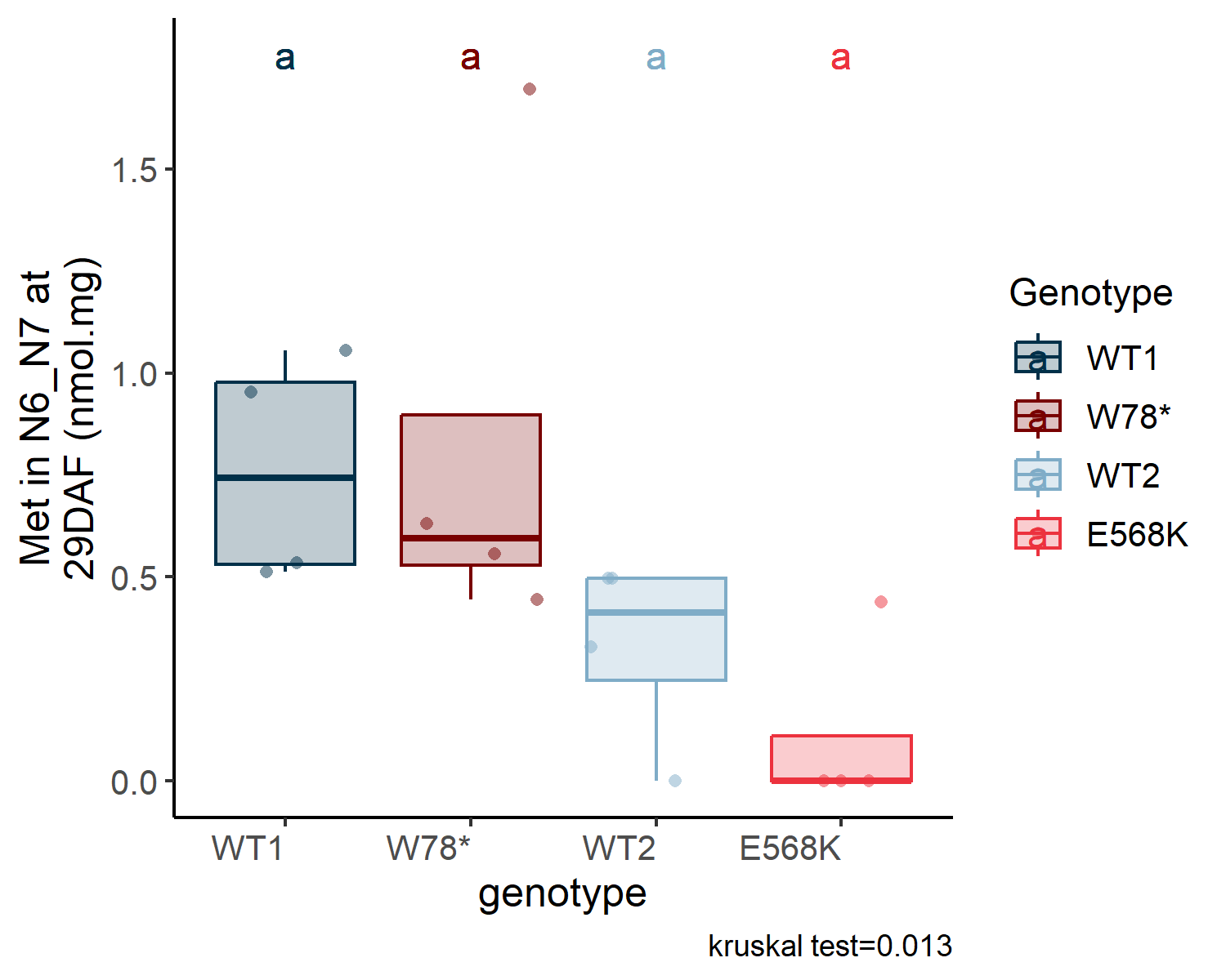
print(final_plot)
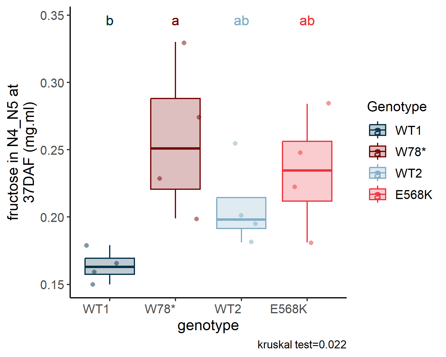
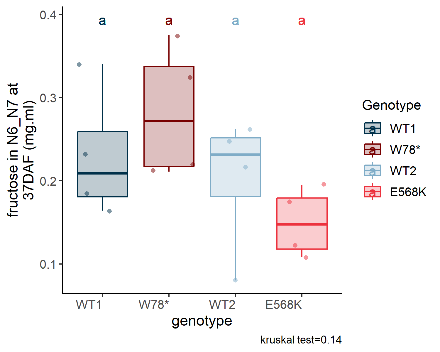
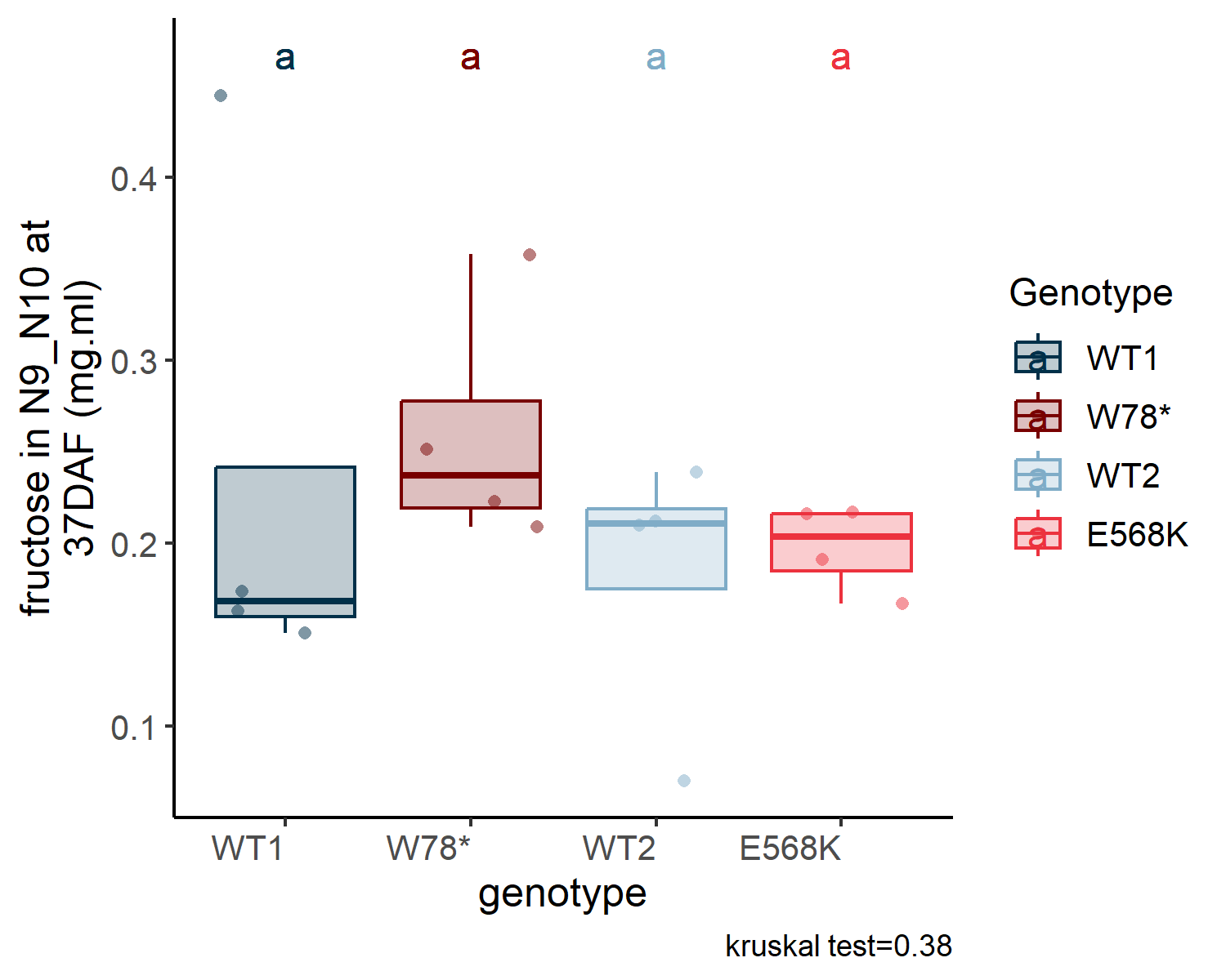
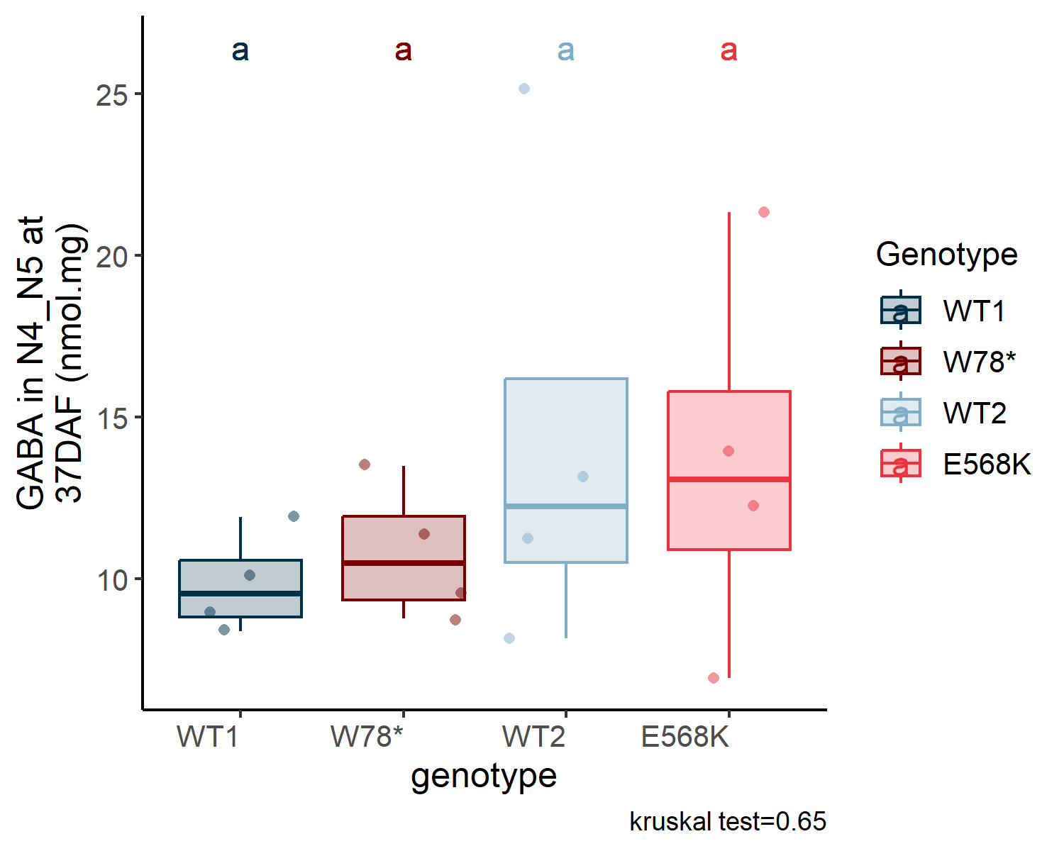
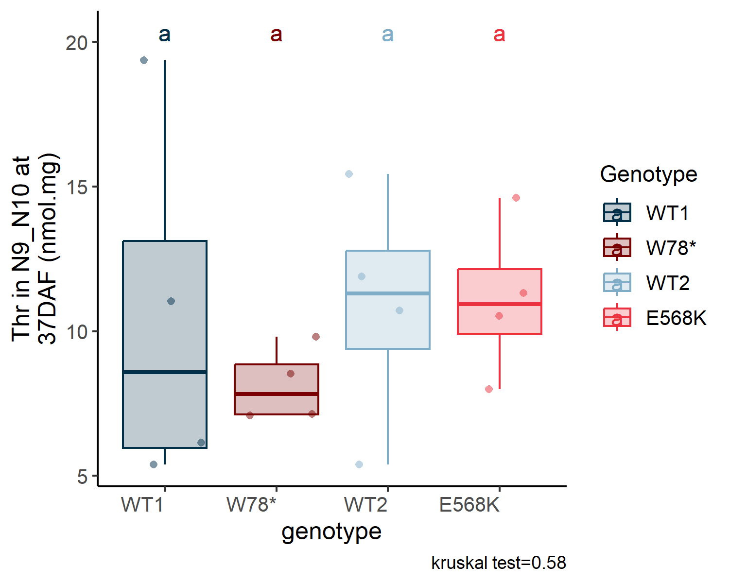
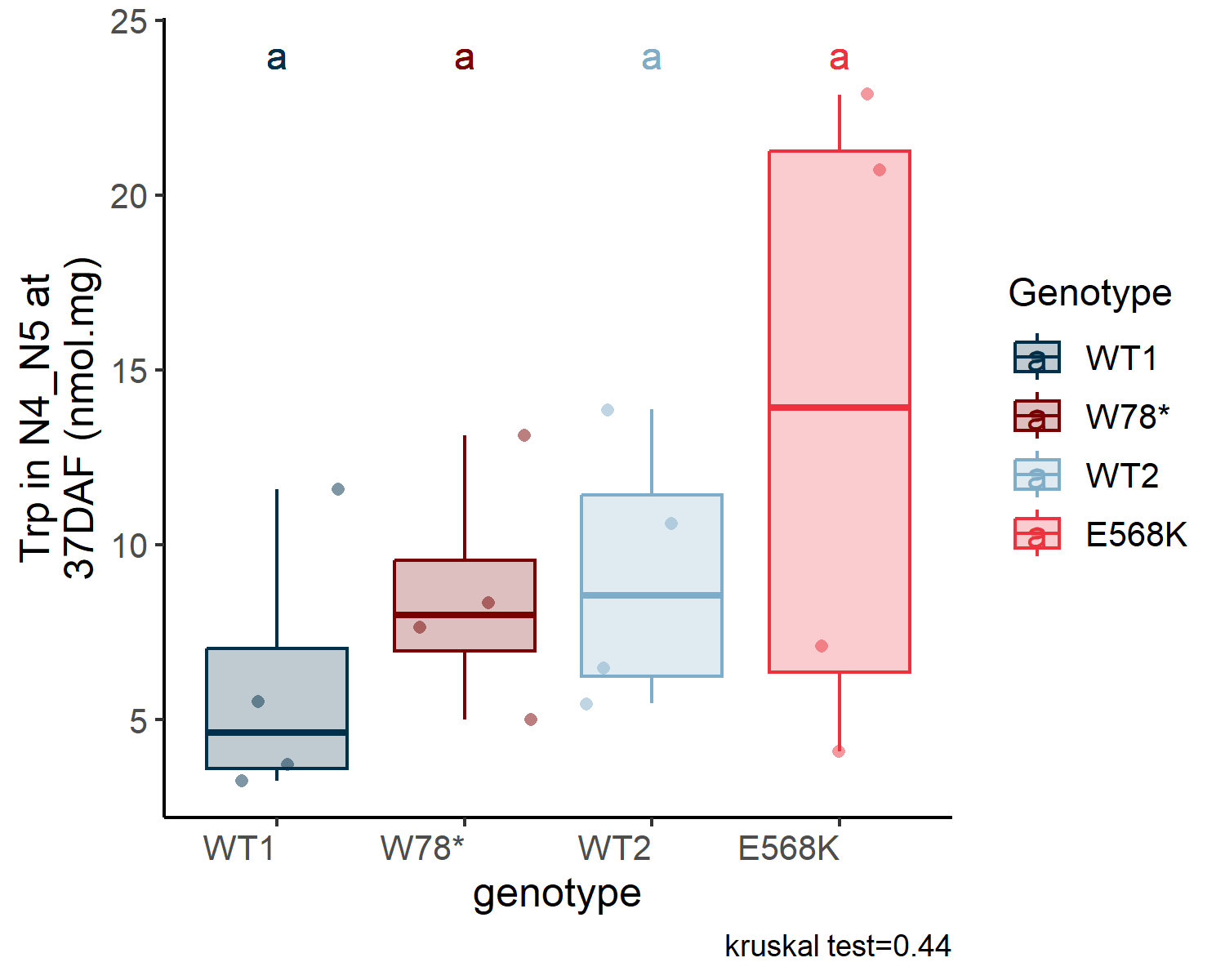
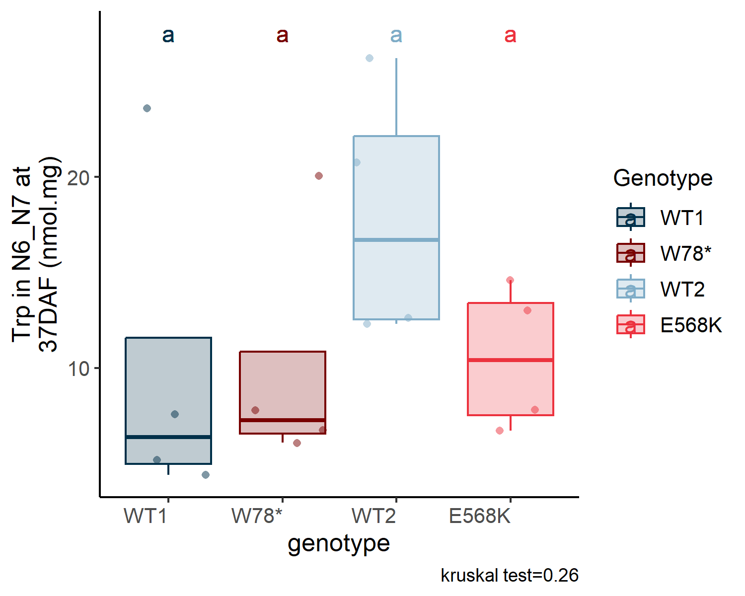
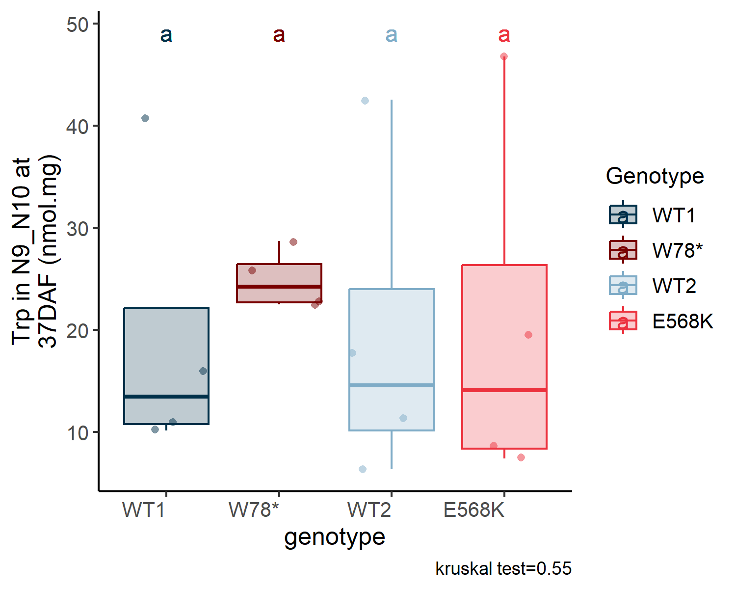
fig_export(here::here("report/metabolomic/plot/SD_metabo_stats"), final_plot, height_i = 28, width_i = 18, res_i = 600)

9.5 Heatmap stats

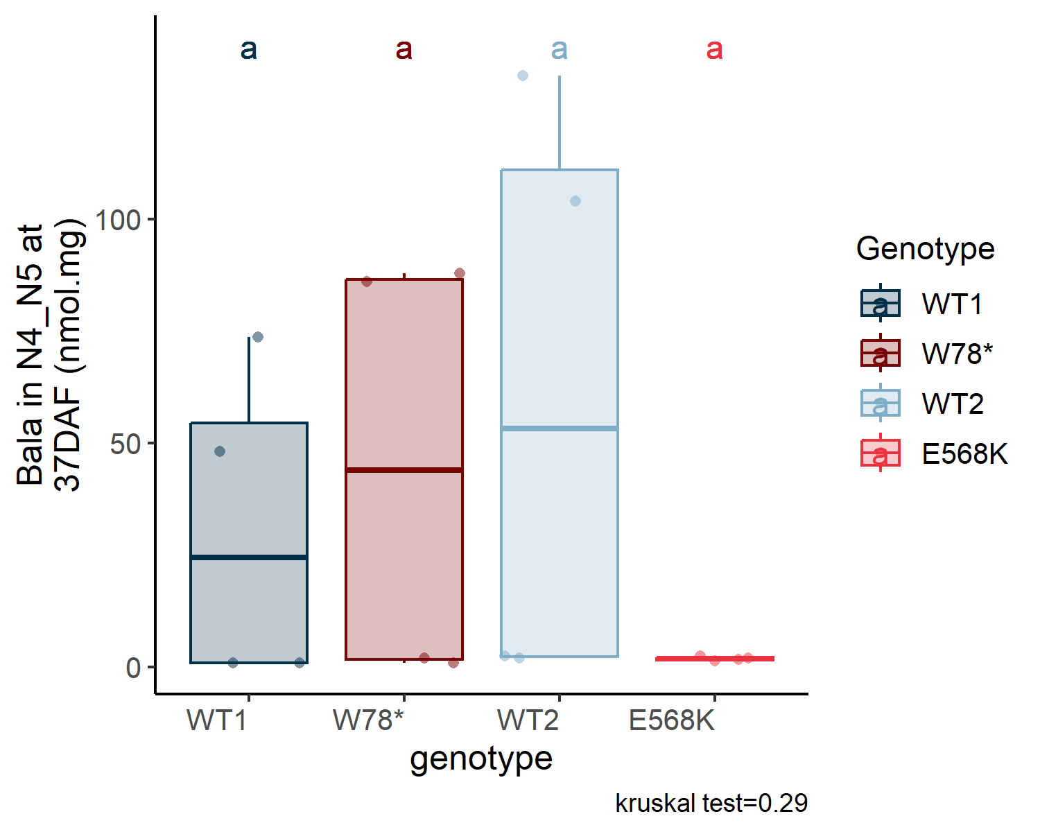
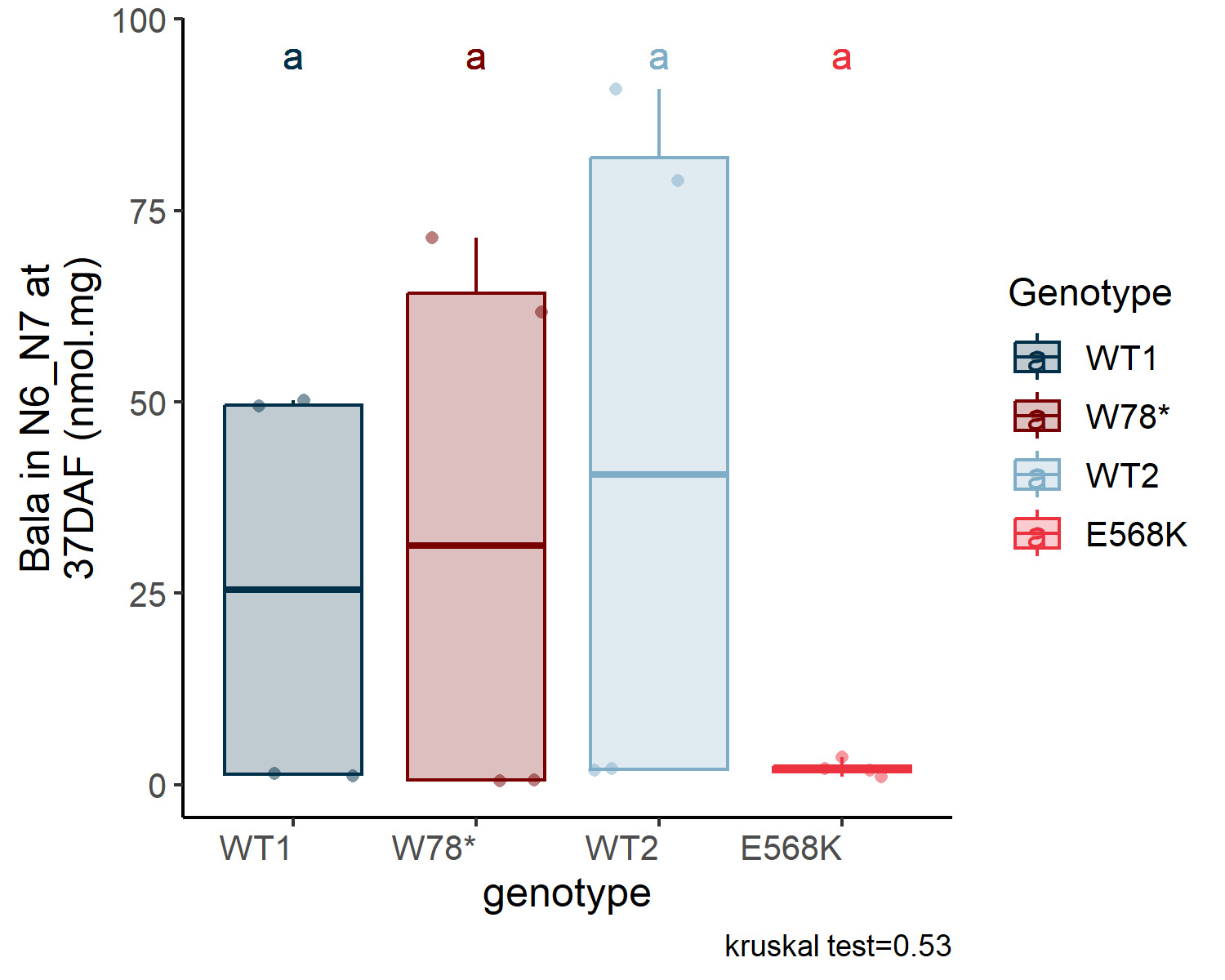
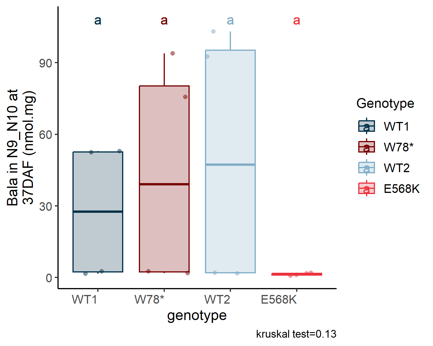
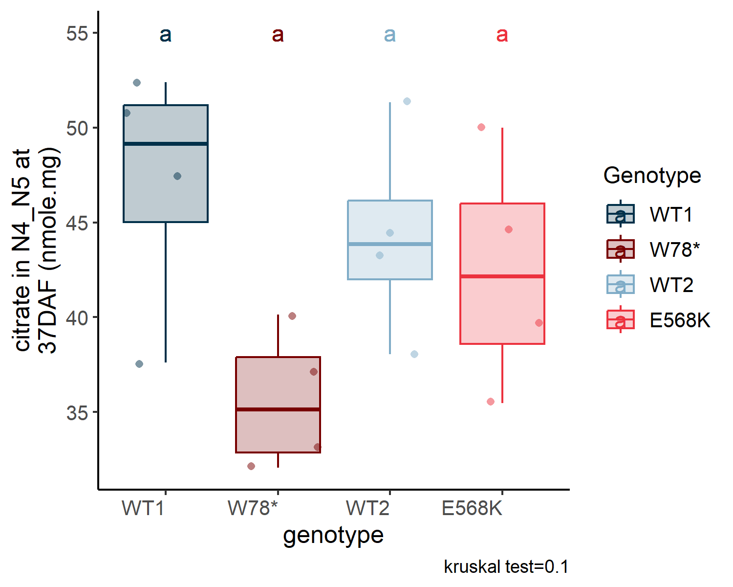
The aim is to create heatmap portions with the stats inside, and then put them back on metabolic pathways.

Code
df_metabolite_global <- read_csv(here::here("data/metabolomic/output/df_metabolite_global.csv"), show_col_types = FALSE) %>% 
  mutate(plant_num = paste(sep = "_", plant_num, condition)) %>% 
  mutate(sulfur_condition= fct_relevel(sulfur_condition, "SS", "SD"),
         genotype = fct_relevel(genotype, "WT1", "W78*", "WT2", "E568K"),
         compartment = fct_relevel(compartment, "N4_N5", "N6_N7"),
         type_genotype = fct_relevel(type_genotype, "WT", "Mut")
         ) %>% 
  filter(sulfur_condition == "SD") %>% 
  filter(!(variable == "Met" & compartment == "N9_N10")) # error of measure/ in WT2 = 0 in all 
  

# input one metabolite
variable_i <- "Asp"
variable_i <- "OAS"
DAF_i <- 29

v_variable <- levels(as.factor(df_metabolite_global %>% filter(DAF==29) %>% distinct(variable) %>% pull(variable)))
#compartment_i <- "N6_N7"

# measure min max of Zscore for color of the graduation
data_for_guides = df_metabolite_global %>% filter(DAF==29) %>% dplyr::group_by(variable) %>%
  dplyr::mutate(value_scaled = as.vector(scale(value))) %>%
  ungroup() %>% 
  dplyr::group_by(variable, genotype) %>% 
  dplyr::summarise(mean_scale = mean(value_scaled))

# min(data_for_guides$mean_scale)
# max(data_for_guides$mean_scale)

for(variable_i in v_variable){
  # variable_i <- "OAS"
  # variable_i <- "Asp"
  # filter data
  df_select <- df_metabolite_global %>% 
      filter(
        sulfur_condition == "SD",
        DAF == DAF_i, 
        variable == variable_i#,
        #compartment == compartment_i
      ) %>% 
      drop_na(value) %>% 
      as.data.frame()
  
  # make stats
  combined_res <- list()
  compartment_v <- levels(as.factor(as.character(df_select$compartment)))
  n_compartment_v <- length(compartment_v)
  for (i in compartment_v){
    
    df_select_compartment <-   df_select %>% filter(compartment == i)
    
    ylab_i <-  paste0(variable_i, " in ", i, " at\n", DAF_i, "DAF (",df_select_compartment %>% 
    head(1) %>%
    pull(unit),")")
    
    res <- stat_analyse(
            data = df_select_compartment,
            column_value = "value",
            category_variables = c("genotype"),
            grp_var = "",
            show_plot = TRUE,
            outlier_show = FALSE, 
            label_outlier = "plant_num",
            biologist_stats = TRUE,
            Ylab_i = ylab_i,
            control_conditions = "",
            strip_normale = FALSE,
            hex_pallet =  c("#003049", "#780000", "#7FACC7", "#EC323E")
          )
    
    stats_resum <- res$data_used %>% distinct(genotype, variable, group)
    res_resum_raw <- res$summary_result %>% 
      left_join(.,stats_resum, by = "genotype") %>% 
      mutate(column_value = variable_i)
    
    res_resum <- res$data_used %>% 
      mutate(value_scaled = scale(value)) %>%  # scale based on z-score is beter than force in -1 ; 1
      dplyr::group_by(compartment, genotype, stage, sulfur_condition, type_genotype, type_variable, DAF, unit) %>%
      dplyr::summarise(
        mean_scale = mean(value_scaled),
        .groups = 'drop'
      ) %>% left_join(.,stats_resum, by = "genotype")
    
    combined_res[[i]] <- res_resum
  }
  
  final_res <- bind_rows(combined_res) %>% 
    mutate(color_text = ifelse(mean_scale<0, "white", "black"))
  
  min_max_zscore <- paste0("min:",round(min(final_res$mean_scale),2),";max:",round(max(final_res$mean_scale),2))
  
  # creation of the plot 
  p_plot <- ggplot(final_res, aes(x = genotype, y = compartment, fill = mean_scale)) +
    geom_tile(color = "white") + # Pour dessiner les cases
    geom_text(aes(label = group, color = color_text)) + # Ajouter les lettres statistiques
    scale_fill_gradient2(low = "#1d4877", mid = "#fbb021", high = "#ee3e32", midpoint = (min(data_for_guides$mean_scale)+max(data_for_guides$mean_scale))/2, limits = c(min(data_for_guides$mean_scale),max(data_for_guides$mean_scale)))+# Plage commune entre -2 et 2 pour tous les plots) + # Palette de couleur
    scale_color_manual(values = c("black" = "black", "white" = "white"))+
    theme_minimal() +
    theme(
      axis.title.y = element_blank(), # Supprime le titre de l'axe Y
      axis.title.x = element_blank(), # Supprime le titre de l'axe X
      axis.text.y = element_text(size = 10, face = "bold"), # Style du texte de la variable
      axis.text.x = element_text(size = 12, angle = 90, vjust = +0.5, hjust = 1.0),
      panel.grid.major = element_blank(), # Supprime les grilles
      panel.grid.minor = element_blank()
    ) +
    labs(title = final_res %>% head(1) %>% pull(variable))+
    #guides(fill = guide_colorbar(title = "Mean Value")) ; p_plot
    guides(fill = "none", color = "none") ; p_plot
  
  # export plot
  plot_name <- paste0("DAF",as.character(DAF_i), "_", variable_i)
  fig_export(here::here(paste0("report/metabolomic/plot/for_pathway/", plot_name)), p_plot, height_i = .38*n_compartment_v+0.95, width_i = 2, res_i = 300,format = "svg")
}

#export legend
# Création d'un ggplot minimal uniquement pour la légende
p_legend <- ggplot(final_res, aes(x = genotype, y = compartment, fill = mean_scale)) +
  geom_tile() +
  scale_fill_gradient2(
    low = "#1d4877", 
    mid = "#fbb021", 
    high = "#ee3e32", 
    midpoint = (min(data_for_guides$mean_scale) + max(data_for_guides$mean_scale)) / 2, 
    limits = c(min(data_for_guides$mean_scale), max(data_for_guides$mean_scale))
  ) +
  theme_void() +  # Supprime les axes, titres, etc.
  guides(
    fill = guide_colorbar(title = "Mean Value") # Titre de la légende
  )

# Extraire uniquement la légende
legend <- cowplot::get_legend(p_legend)

# Affichage de la légende seule
grid::grid.newpage()
grid::grid.draw(legend)


fig_export(here::here(paste0("report/metabolomic/plot/for_pathway/legend")), legend, height_i = 2, width_i = 1, res_i = 300,format = "svg")

9.6 Miniboxplot for publication

Code
# data importation
df_metabolite_global <- read_csv(here::here("data/metabolomic/output/df_metabolite_global.csv"), show_col_types = FALSE) %>%
   mutate(
    plant_num        = paste(sep = "_", plant_num, condition),
    sulfur_condition = fct_relevel(sulfur_condition, "SS", "SD"),
    genotype         = fct_relevel(genotype, "WT1", "W78*", "WT2", "E568K"),
    compartment      = fct_relevel(compartment, "N4_N5", "N6_N7"),
    type_genotype    = fct_relevel(type_genotype, "WT", "Mut"),
    condition        = paste0(sulfur_condition, "_", genotype),

    # --- NEW COLUMN ---
    genotype2 = if_else(
      sulfur_condition == "SS" & genotype %in% c("WT1", "WT2"),
      "WT",
      as.character(genotype)   # keep original name otherwise
    ),
    condition2 = paste0(sulfur_condition, "_", genotype2)
  ) %>% 
  filter(!(variable == "Met" & compartment == "N9_N10")) %>%  # error of measure/ in WT2 = 0 in all
  filter(compartment == "N9_N10") %>% 
  filter(DAF == 29) 

v_variable <- df_metabolite_global %>% distinct(variable) %>% pull(variable)
for (i in v_variable){
# variable_i = "Sulfate"
variable_i = i
df_select <- df_metabolite_global %>% 
  filter(variable == variable_i) %>% 
      drop_na(value) %>% 
      as.data.frame()
  
ylab_i <-  paste0(variable_i, " in vegetative leaves (", df_select$unit[1], ")")
    
res <- stat_analyse(
  data = df_select,
  column_value = "value",
  category_variables = c("condition2"),
  grp_var = "",
  show_plot = TRUE,
  outlier_show = FALSE, 
  label_outlier = "plant_num",
  biologist_stats = TRUE,
  Ylab_i = ylab_i,
  control_conditions = "",
  strip_normale = FALSE,
  hex_pallet =  c(as.character(sulfate_pallet[1]),  "#003049", "#780000", "#7FACC7", "#EC323E")
  )

p_res <-res[["plot"]]+theme(legend.position = "none", 
                                             axis.text.x = element_text(
                                               angle = 90,
                                               vjust = 0.5,
                                               hjust = 1))+
                                             labs(color = "Condition", fill = "Condition", x = "")

fig_export(here::here(paste0("report/metabolomic/plot/for_pathway_boxplot/", variable_i, "_DAF29_N9N10")), p_res, height_i = 4.2, width_i = 2.2, res_i = 300,format = "svg")
}